This guide will show you how to generate vector-based topopgraphic maps, for printing very large & high-quality paper wall maps using inkscape. All of the tools used in this guide are free (as in beer).
Intro
I recently volunteered at a Biological Research Station located on the eastern slopes of the Andes mountains. If the skies were clear (which is almost never, as it’s a cloud forest), you would have a great view overlooking the Amazon Rainforest below.
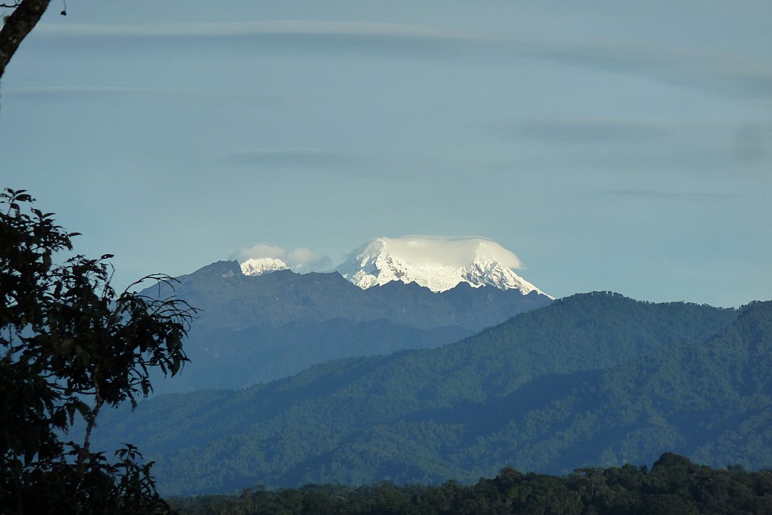
Yanayacu is in a cloud forest on the east slopes of the Andes mountains, just 30 km from the summit of the glacial-capped Antisana volcano (source)
The field station was many years old with some permanent structures and a network of established trails that meandered towards the border of Antisana National Park – a protected area rich with biodiversity that attracts biologists from around the world. At the top of the park is a glacial-capped volcano with a summit at 5,753 meters.
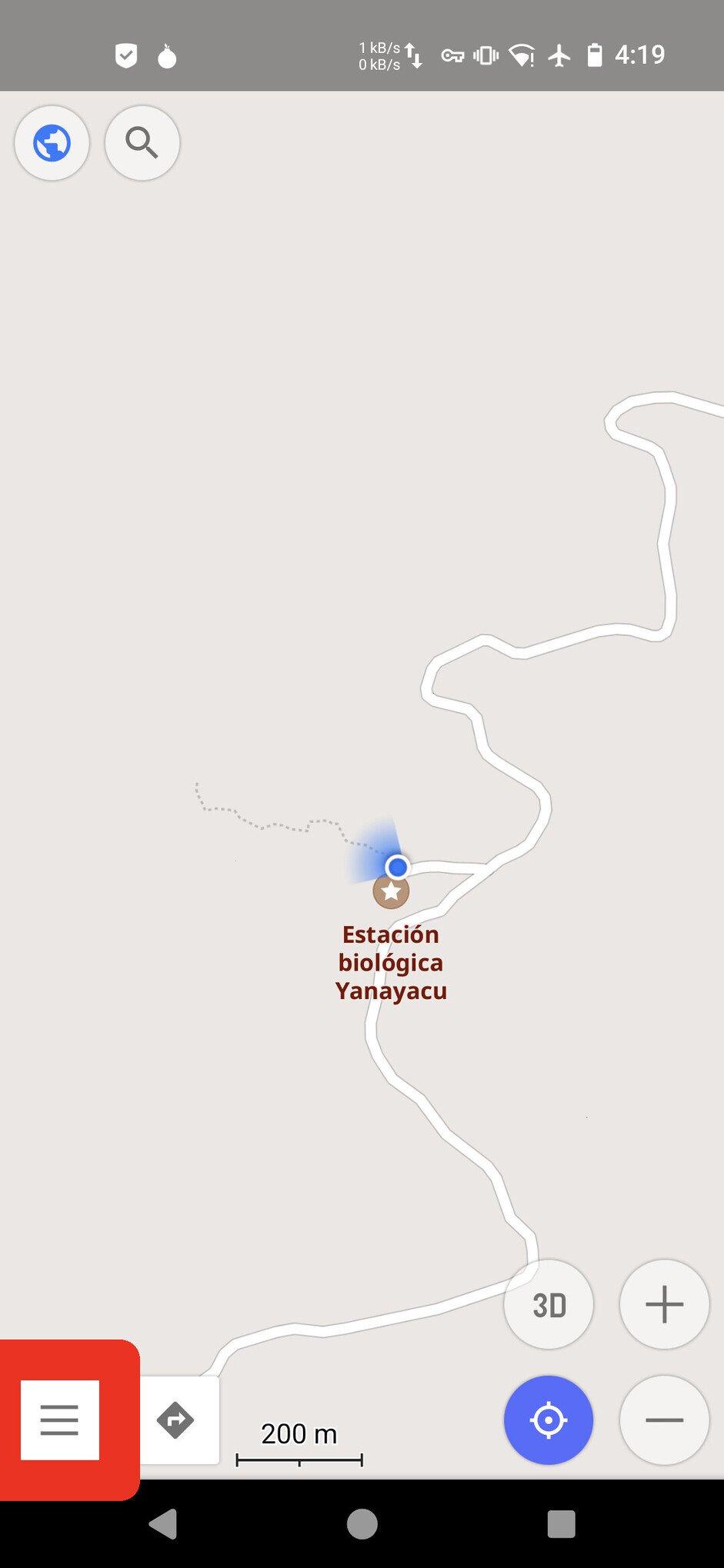
Surprisingly, though Estacion Biologicia Yanayacu was over 30 years old, nobody ever prepared a proper map of their trails. And certainly there was no high-resolution topographical map of the area to be found at the Station.
That was my task: to generate maps that we could bring to a local print shop to print-out huge 1-3 meter topographical maps.
And if you want to print massive posters that don’t look terrible, you’re going to be working with vector graphics. However, most of the tools that I found for browsing Open Street Map data that included contour lines couldn’t export an SVG. And the tools I found that could export an SVG, couldn’t export contour lines.
It took me several days to figure out how to render a topographical map and export it as an SVG. This article will explain how, so you can produce a vector-based topographical map in about half a day of work.
Assumptions
This guide was written in 2024, and it uses the following software and versions:
- Debian 12 (bookworm)
- OsmAnd~ v4.7.10
- JOSM v18646
- Maperitive v2.4.3
- Inkscape v1.2.2
You will likely encounter bugs, and — because the original author is hostile to free software — nobody can update it 🙁 You may want to look into using QGIS instead.
The Tools
Unfortunately, there’s no all-in-one app that will let you just load a slippy map, zoom-in, draw a box, and hit “export as SVG”. We’ll be using a few different tools to meet our needs.
![[OsmAnd]](https://tech.michaelaltfield.net/wp-content/uploads/sites/5/xosm-contours-svg-maperitive_osmand-icon1-150x150.jpg.pagespeed.ic.RKAvG3SHn5.jpg)
OsmAnd
OsmAnd is a mobile app.
We’ll be using OsmAnd to walk around on the trails and generate GPX files (which contain a set of GPS coordinates and some metadata). We’ll use these coordinates to generate vector lines of a trail overlaying the topographic map.
If you just want a topographic map without trails (or your trails are already marked on OSM data), then you won’t need this tool.
In this guide we’ll be using OsmAnd, but you an also use other apps — such as Organic Maps, Maps.me, or Gaia.
![[JOSM]](https://tech.michaelaltfield.net/wp-content/uploads/sites/5/xosm-contours-svg-maperitive_josm-icon1-150x150.jpg.pagespeed.ic.ke9ufFzzUG.jpg)
JOSM
JOSM is a java-based tool for editing Open Street Map data.
We’ll be using JOSM to upload the paths of our trails (recorded GPX files from OsmAnd) and also to download additional data (rivers, national park boundary line, road to the trailhead, etc). We’ll then be able to combine all of this data into a larger GPX file, which will eventually become vector lines overlaying the topographic map.
You can skip this if you just want contour lines without things like rivers, roads, trails, buildings, and park borders.
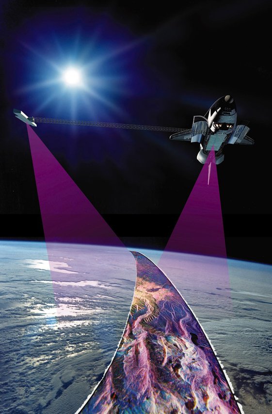
This illustration shows the Space Shuttle Endeavour orbiting ~233 kilometers above Earth. The two anternae, one located in the Shuttle bay and the other located on a 60-meter mast, were able to penetrate clouds, obtaining 3-dimentional topographic images of the world’s surface (source: NASA)
View Finder Panoramas
Have you ever wondered how you can zoom-in almost anywhere in the world and see contour lines? I always thought that this was the result of some herculean effort of surveyors scaling mountains and descending canyons the world-over. But, no — it’s a product of the US Space Shuttle program.
In the year 2000, an international program called SRTM (Shuttle Radar Topography Mission) was launched into space with the Endaevor Space Shuttle. It consisted of a special radar system tethered to the shuttle with a 60 meter mast as it orbited the earth.
When the shuttle returned to earth, the majority of our planet’s contours were mapped. This data was placed on the public domain. Today, it is the main data source for elevation data in most maps.
While the data from SRTM was a huge boon to cartographers, it did have some gaps. Namely: elevation data was missing in very tall mountains and very low canyons. Subsequent work was done to fill-in these gaps. One particular source that ingested the SRTM data, completed its gaps, and made the results public is Jonathan de Ferranti’s viewfinderpanoramas.org.
We will be downloading .hgt files from View Finder Panoramas in order to generate vector contour lines for our topographical map.
![[Maperitive]](https://tech.michaelaltfield.net/wp-content/uploads/sites/5/xosm-contours-svg-maperitive_maperitive-icon1.jpg.pagespeed.ic.PCuQoJR79g.jpg)
Maperitive
Maperitive is a closed-source .NET-based mapping software (which runs fine in Linux with mono).
We’ll be using Maperitive to tie together our GPX tracks, generate contour lines, generate hillshades, and export it all as a SVG.
![[Inkscape]](https://tech.michaelaltfield.net/wp-content/uploads/sites/5/xosm-contours-svg-maperitive_inkscape-icon1-150x150.jpg.pagespeed.ic.khU2rFDNyn.jpg)
Inkscape
Inkscape is a cross-platform app for artists working with vector graphics.
We’ll be using inkscape to make some final touches to our vector image, such as hiding some paths, changing their stroke color/shape/thickness, and adding/moving text labels. Finally, we’ll use inkscape to export a gigantic, high-definition .png raster image (to send to the print shop).
Guide
This section will describe how to make the map.
Walk the Walk
Most of the work to make a map will be done in-front of a computer screen, but—if you want to map a trail—first you gotta walk the walk.
Check the weather. Wear good boots. Pack your lunch. Bring a rain coat. Make sure your phone is fully charged.
Download OsmAnd and the offline maps of your area. Enable the Trip recording plugin.
-
- Click on the hamburger icon to open the menu

-
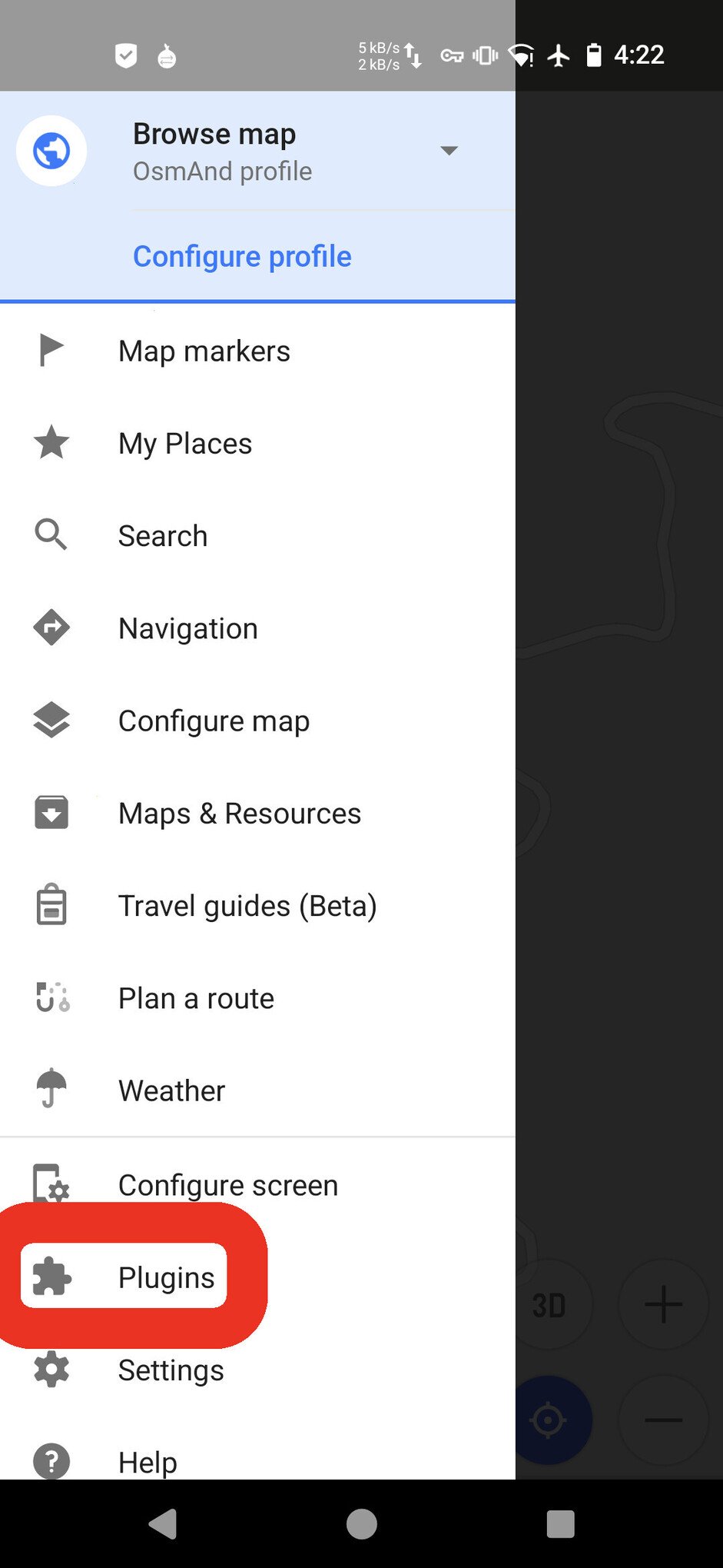
- Click “Plugins”

-

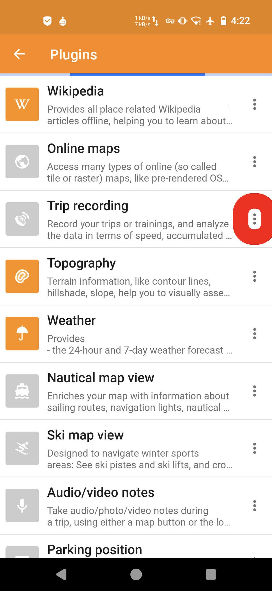
- Click the menu button next to “Trip recording”
-
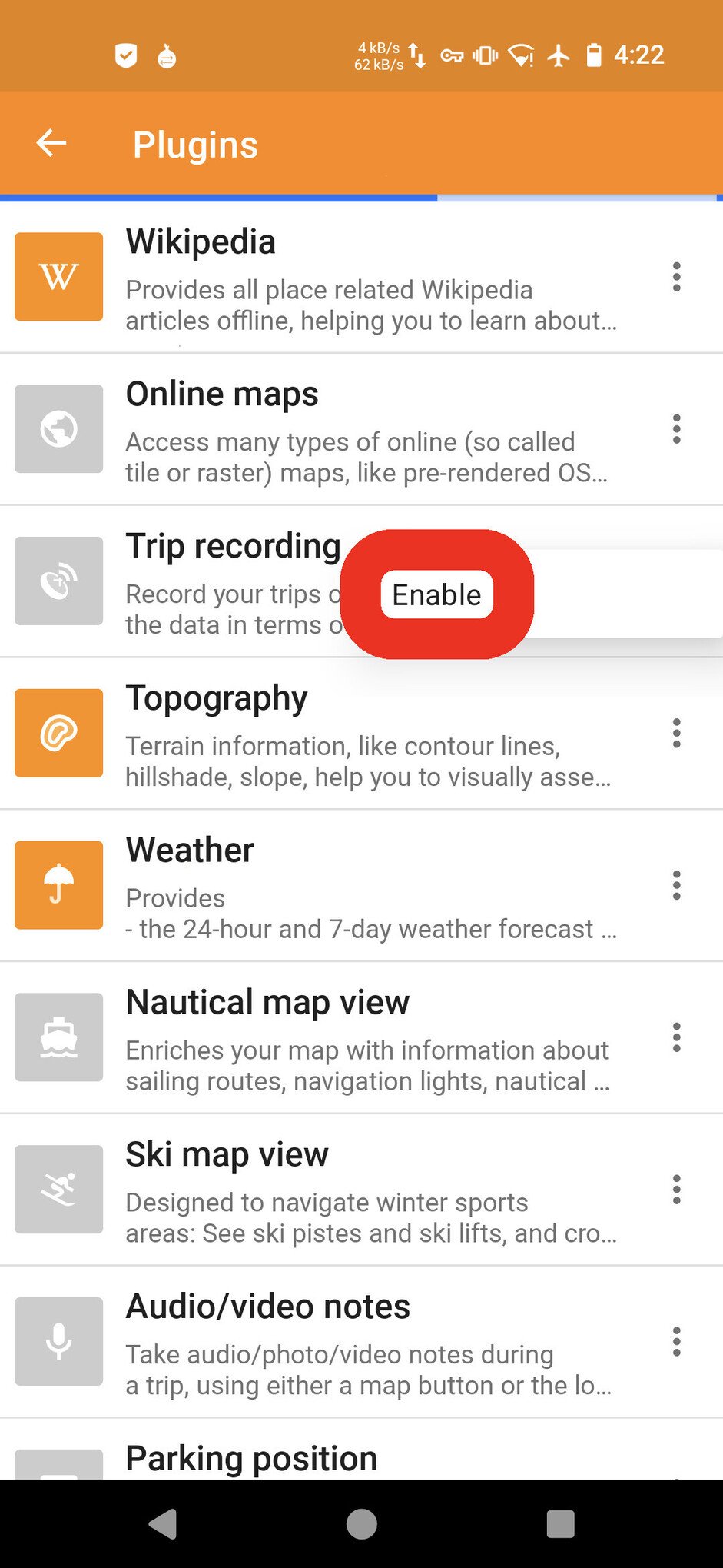
- Click “Enable”

-

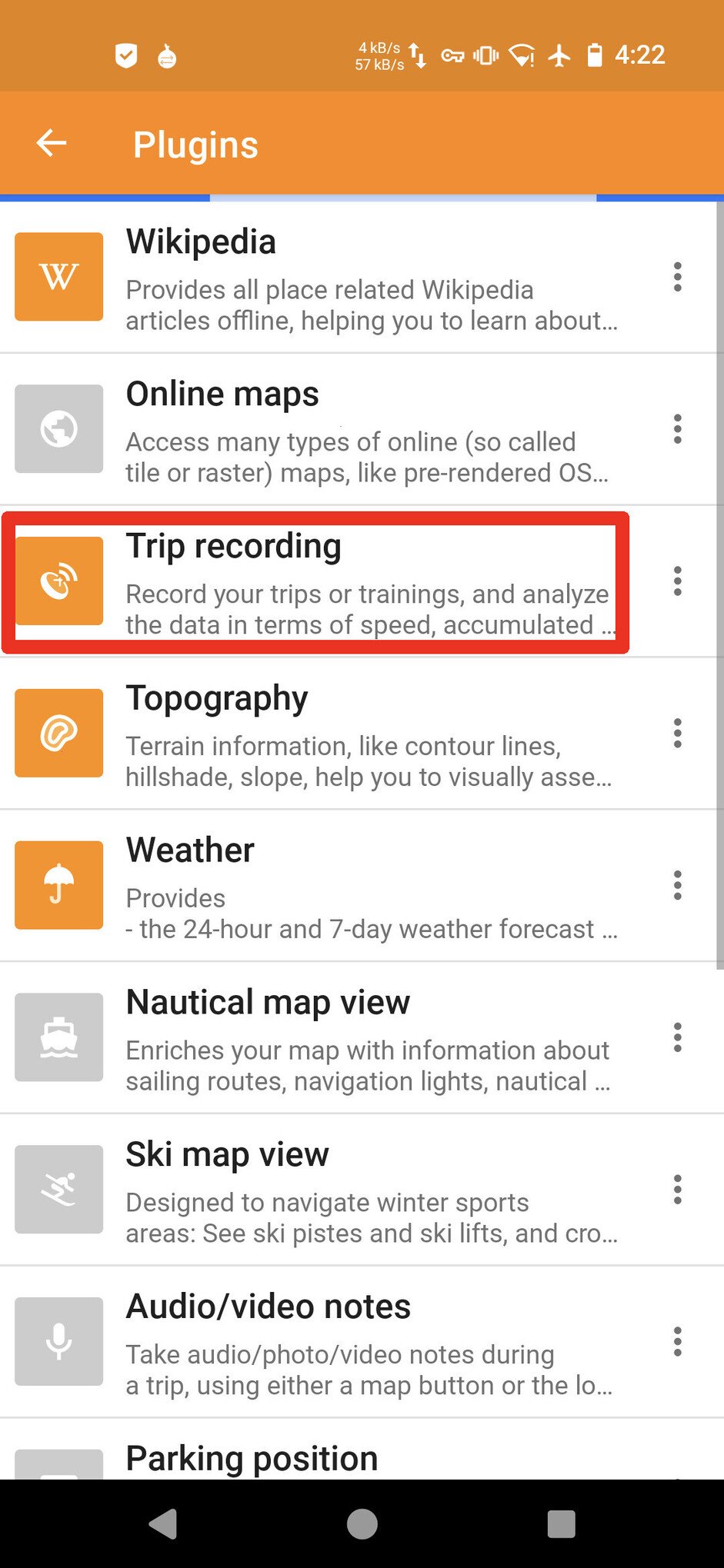
- When the plugin is enabled, its icon will change from grey to orange
When you arrive to the trailhead, open OsmAnd and wait for a GPS lock. Then press the “REC” button, make sure “Show on map” is enabled, and tap “Start”.
-

- Click “REC” to begin recording a GPX track
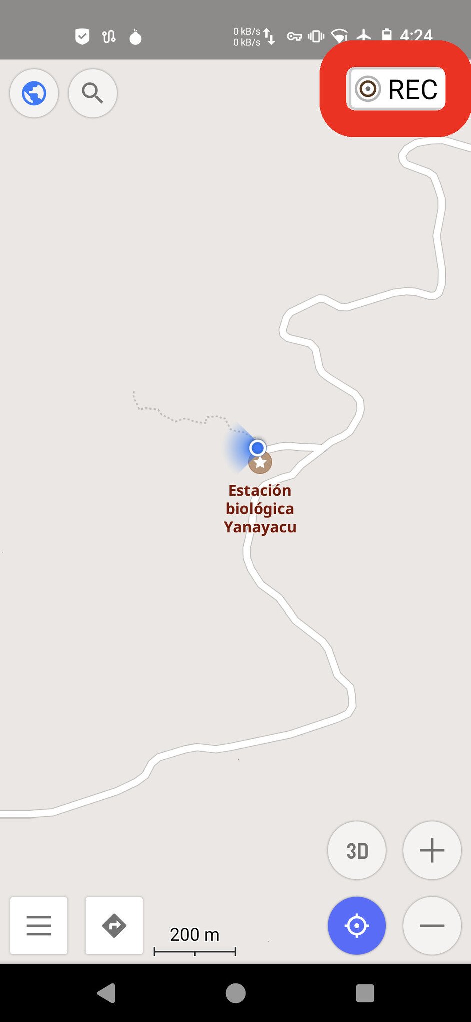
-
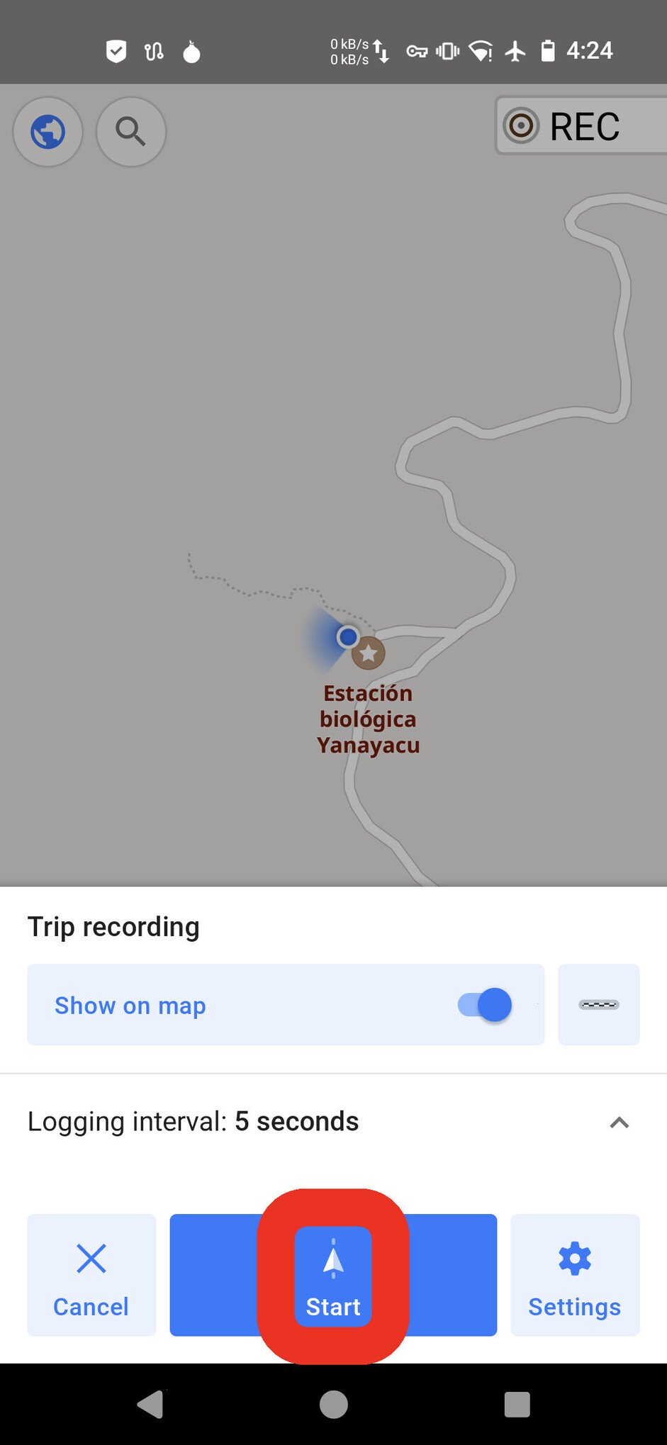
- Click “Start”

If this is your first time doing this, then I do recommend checking your phone periodically to make sure that a line tracing your walking path is overlaying the map. It’s possible that your OS is set to conserve your battery, which might turn off your GPS module when the phone is in your pocket.
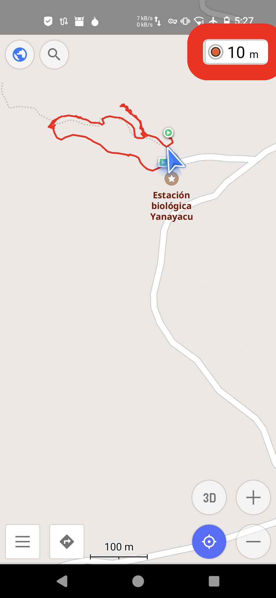
Take your time. Enjoy yourself. But try not to walk off-path (your GPS will track that and it may be confusing to you later).
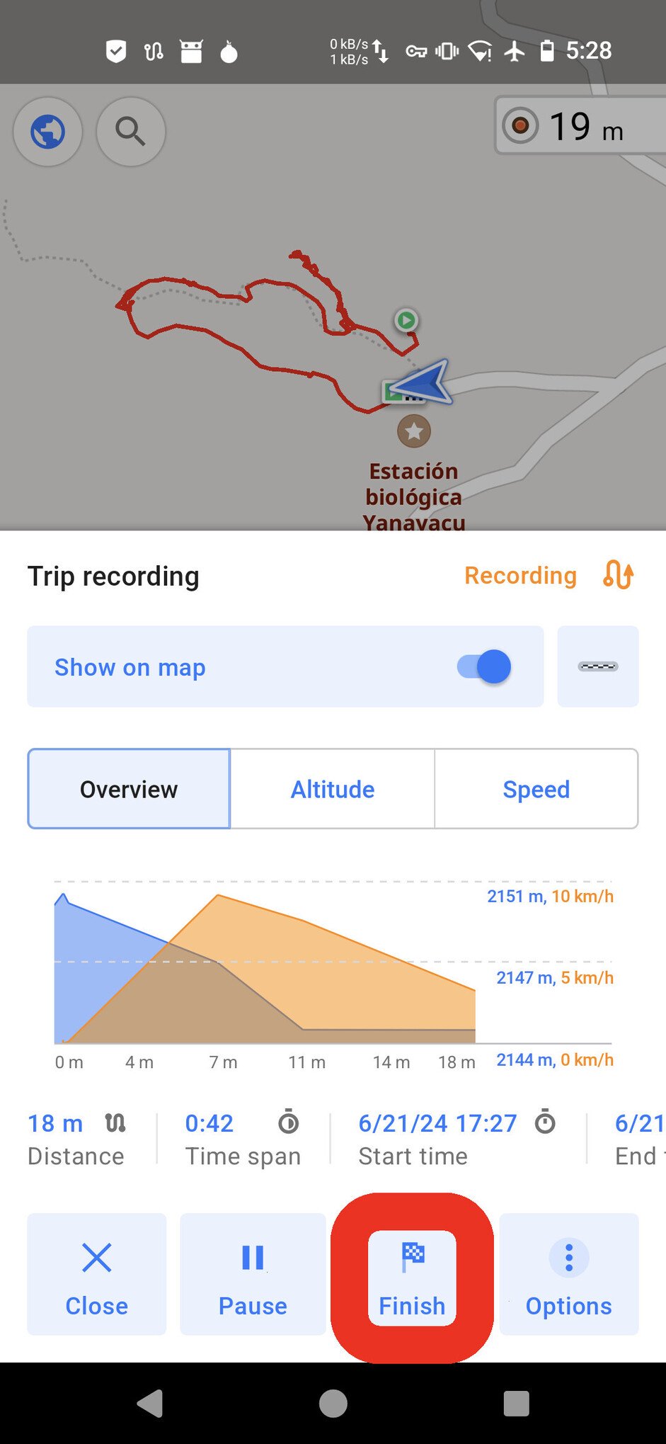
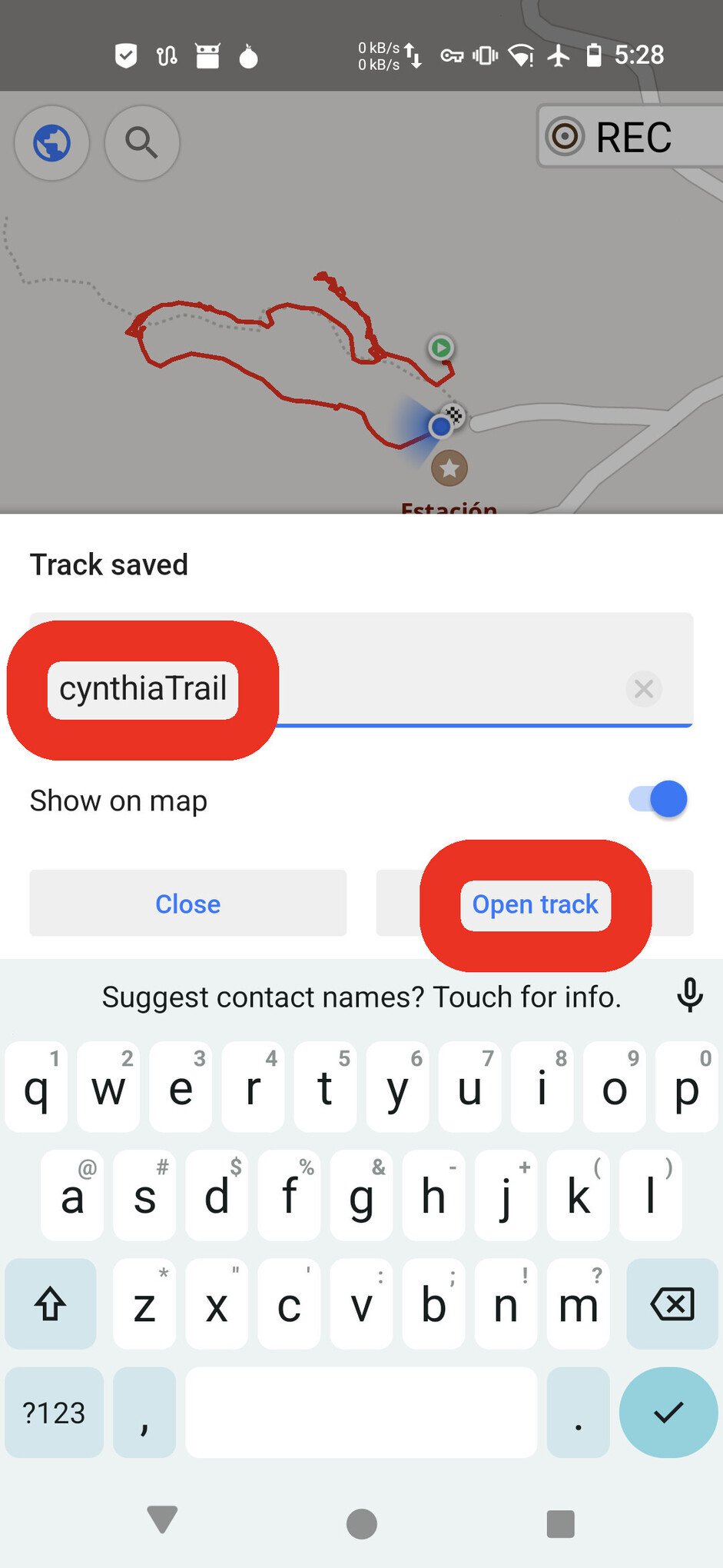
When you’ve reached the end of the trail, click the “REC(ord)” button again (which now will say the distance of your track, but still have a red “recording” icon) and tap “Finish”. Give it a name.
-
- Click on the red “recording” icon to stop and save your GPX track

-

- Click “Finish”
-

-
Type a name for your
.gpxfile, and click “Open track”
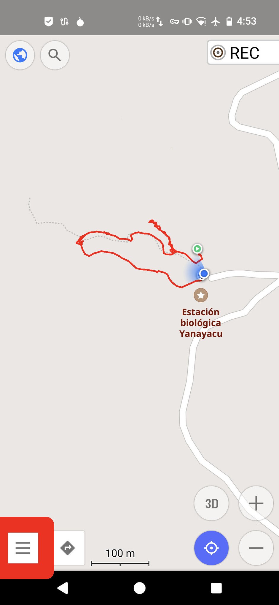
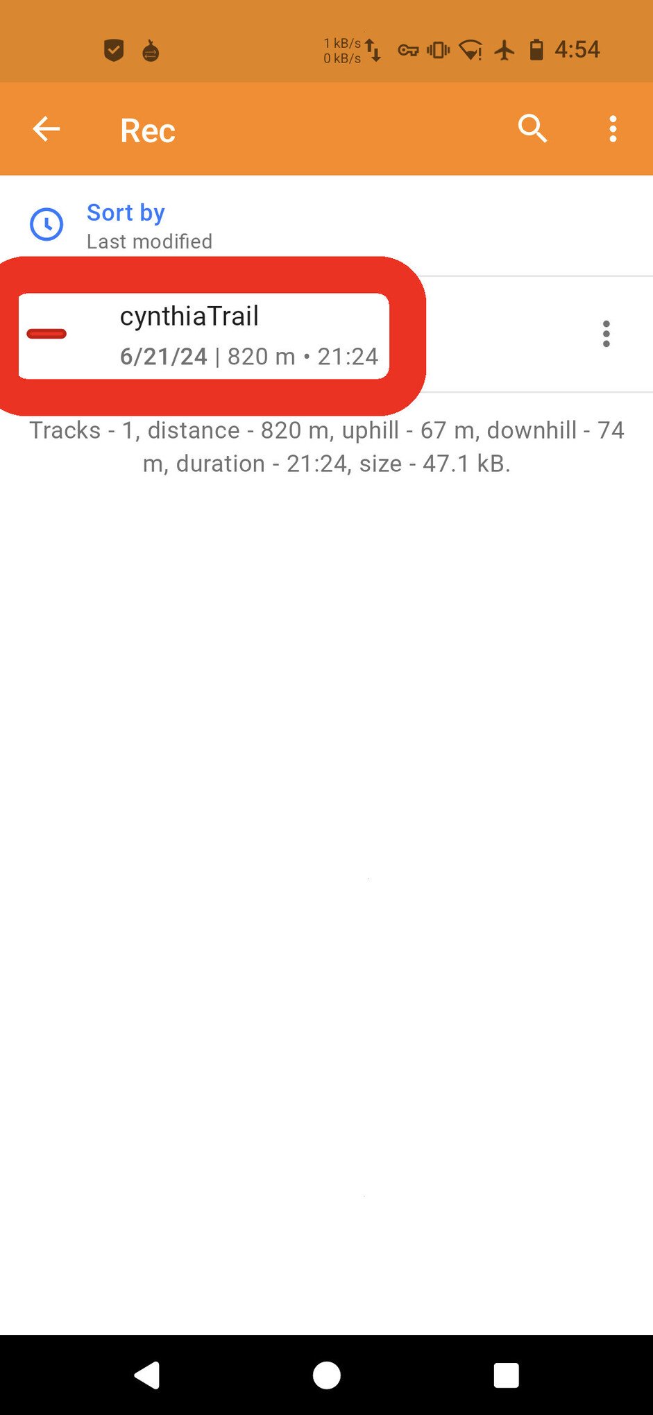
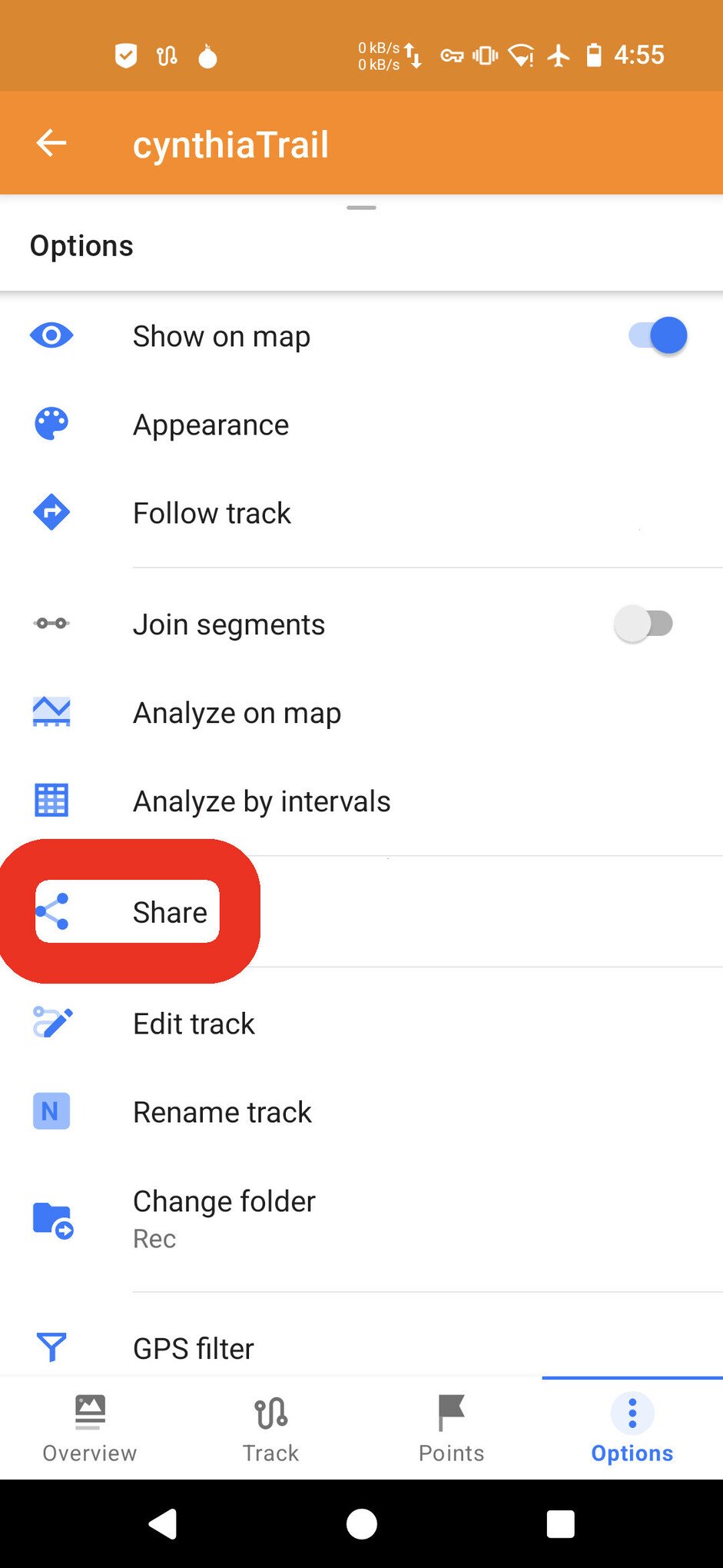
Later, when you’ve returned to your computer desk, you can export the path of your walk that you just recorded as a .gpx file by going to the OsmAnd Menu -> My Places -> Rec. Tap on the name of the trace, then click options -> Share.
-
- Click on the hamburger icon to open the menu

-
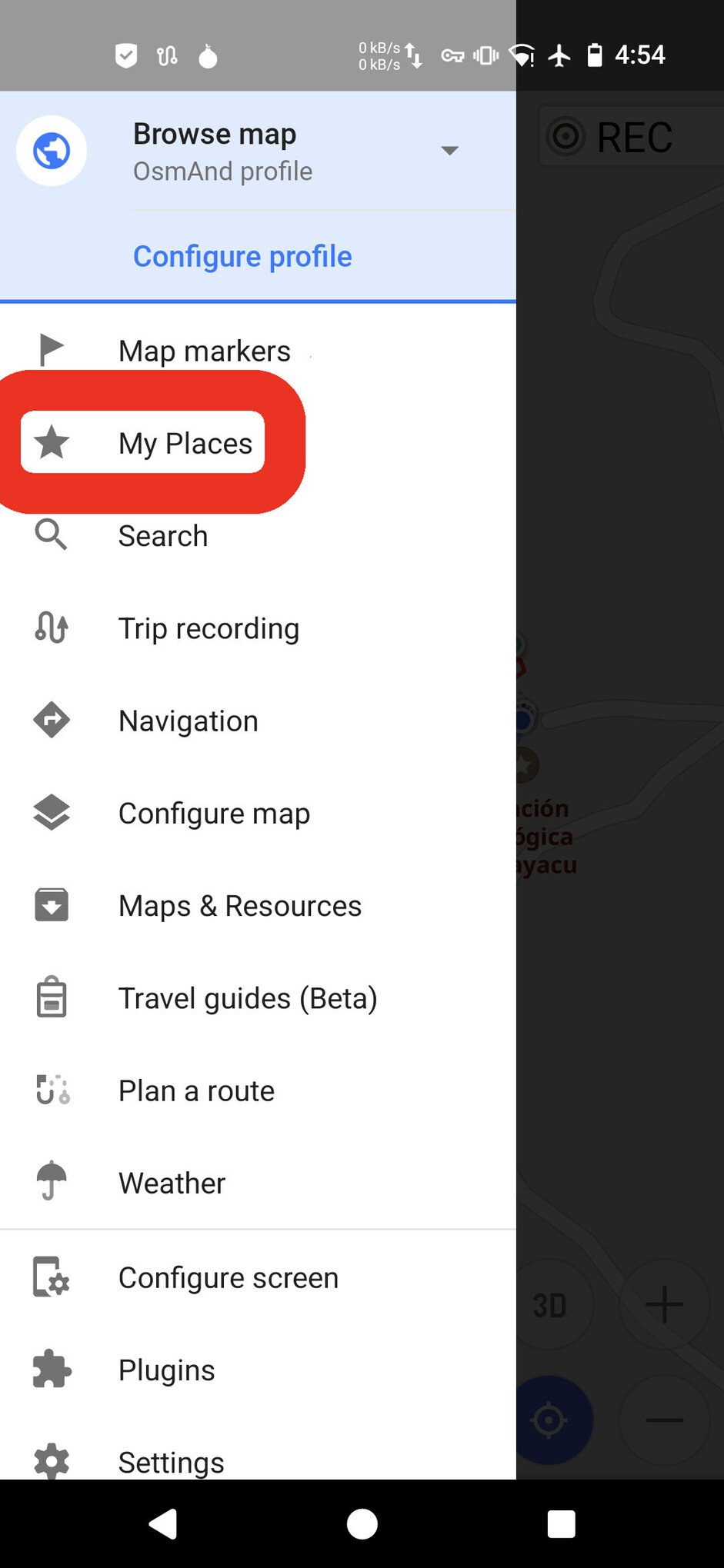
- Click “My Places”

-
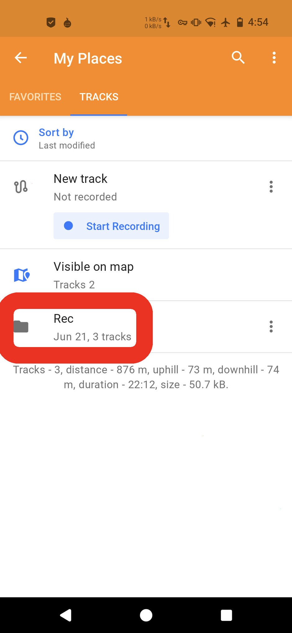
- Click “Rec”

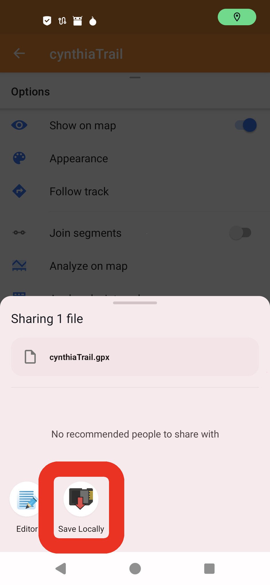
I typically share it with the Save Locally app in order to save it to my phone’s disk.
-

- Click on the name of the GPX track that you want to export
-
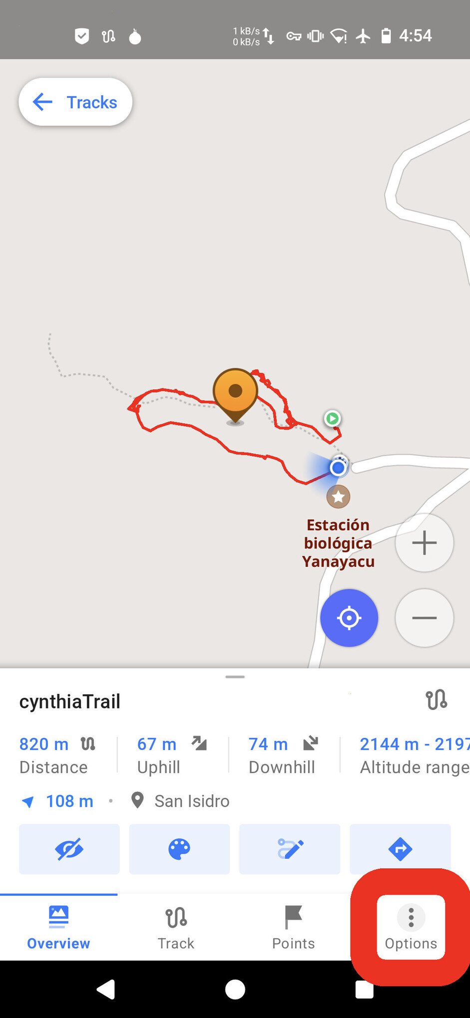
- Click “Options”

-

- Click “Share”
-
-
I use the Save Locally app to save the
.gpxfile to disk

Copying files from your phone to your computer is outside the scope of this article, but you could either use a cable, sdcard, or apps like OnionShare or Syncthing.
Downloading and Editing GPX Tracks
Next, let’s open our .gpx tracks on the computer and also download paths of other user-contributed data about the same area from Open Street Map (eg the path of rivers, roads, and other trails).
Install JOSM
I think the best cross-platform tool to download and edit OSM data is JOSM. There’s a few ways to install it in Debian.
JOSM is in the default repos, but it will give you an older version.
# this is the best and safest way to install JOSM
sudo apt-get install josm
If you want a newer version, you can also install JOSM from the official Debian backports repo.
cat << EOF | sudo tee /etc/apt/sources.list.d/backports.list
deb http://deb.debian.org/debian bookworm-backports main
EOF
sudo apt-get update
sudo apt-get install -t bookworm-backports josm
Lastly, you can just download and run the latest version. But I would only do this in some ephemeral & sandboxed VM, since it’s not safe.
⚠ WARNING: Downloading and installing software outside of
aptis not recommended. By default,aptwill cryptographically verify the authenticity of everything that it downloads (since 2005) before installing it. Whereas downloading a.jar(even with https) could lead to you installing malicious software.If you must download software without verifying its authenticity (eg with PGP signatures), then you should at least check it with 3TOFU.
# WARNING: this is not safe and could download malicious code!
wget https://josm.openstreetmap.de/josm-tested.jar
java -jar josm-tested.jar
Downloading Data in JOSM
Open JOSM with the josm command.
user@disp4463:~$ josm
Using /usr/lib/jvm/java-17-openjdk-amd64/bin/java to execute josm.
...
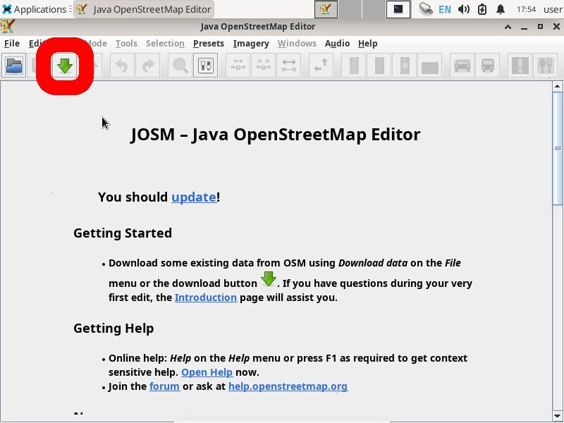
After opening JOSM, click the “Download” button.
-
- First, we download OSM data

-
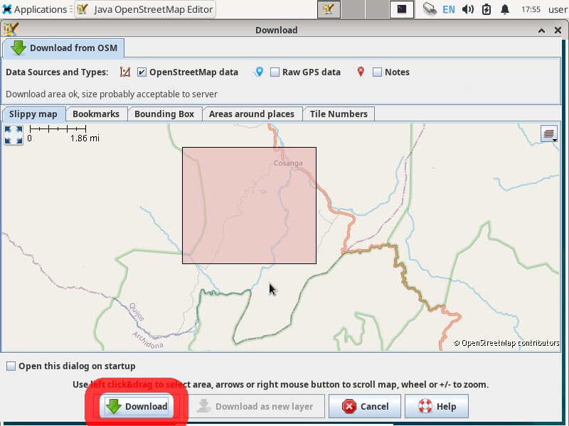
- Draw a box around the area you’re mapping, and click “Download”

Pan the world map to your area of interest using the arrow buttons, and then zoom-in with your mouse wheel (or touchpad scroll gesture). Left-mouse-click and drag to draw a red box that highlights the area where you want to make a map. Then click “Download” to download the OSM data within the box.
Import Data into JOSM
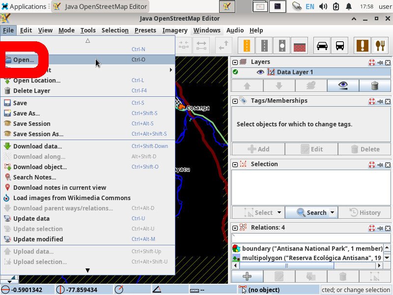
Click the “Open” button.
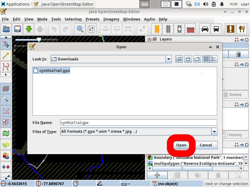
Browse to the GPX file that you copied from your phone, select it, and click the “Open” button.
Edit Data in JOSM
After opening your .gpx file in JOSM, a new row will appear in the Layers List panel. Right-click on this new layer and choose “Convert to data layer“.
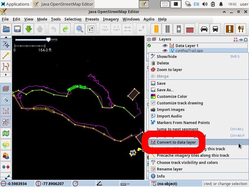
Right Click -> Convert to data layer
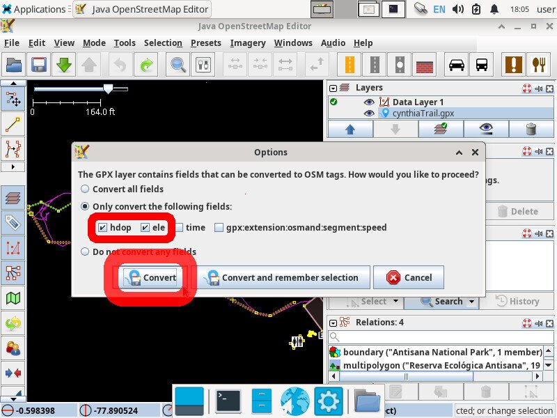
For privacy, I usually only convert the name, elevation, and accuracy metadata of my points.
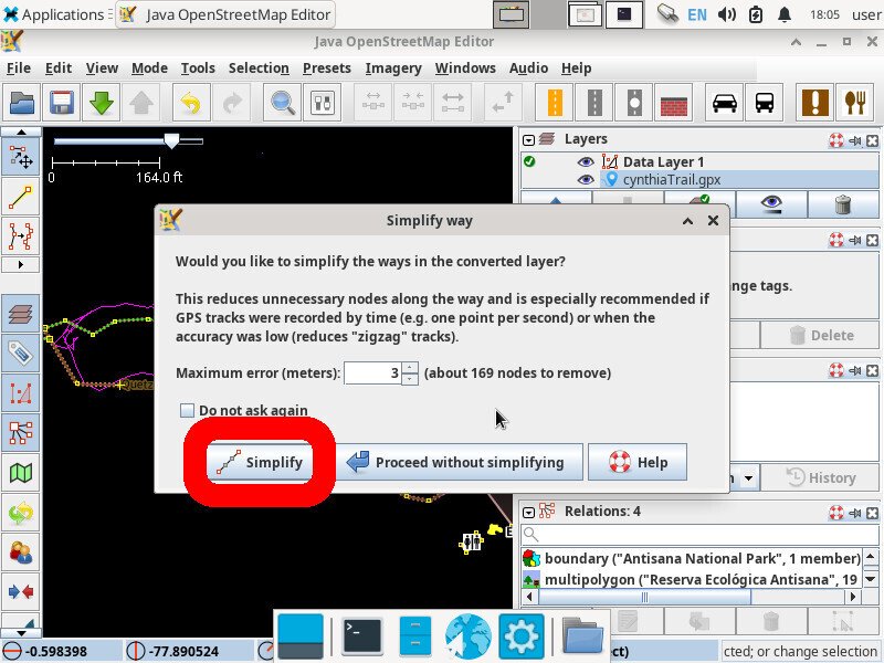
You’ll likely want to have JOSM automagically “simplify” your tracks. I usually take the default of one point every 3 meters.
Now your GPX track should be a set of points connected by lines. You can click on any point to move or delete it. I recommend spending some time “cleaning up” your track (such as removing the trace of you walking in circles at the trailhead or that time you went off-trail to pee).
-
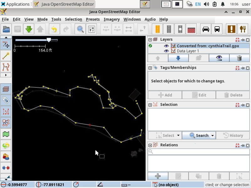
- Spend some time “cleaning up” your gpx track

-

- Very clean 🙂
For more information on editing a way in JOSM, see the official JOSM documentation.
(optional) upload your trail to OSM’s public data set
Optionally, after you edited the trail, you can use JOSM to upload it to be publicly available in the OSM data set. To do so, you’ll want to signup for an OSM account and click the upload button in JOSM.
Export Data from JOSM
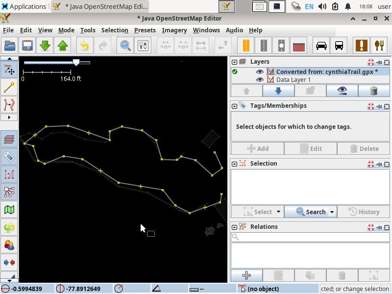
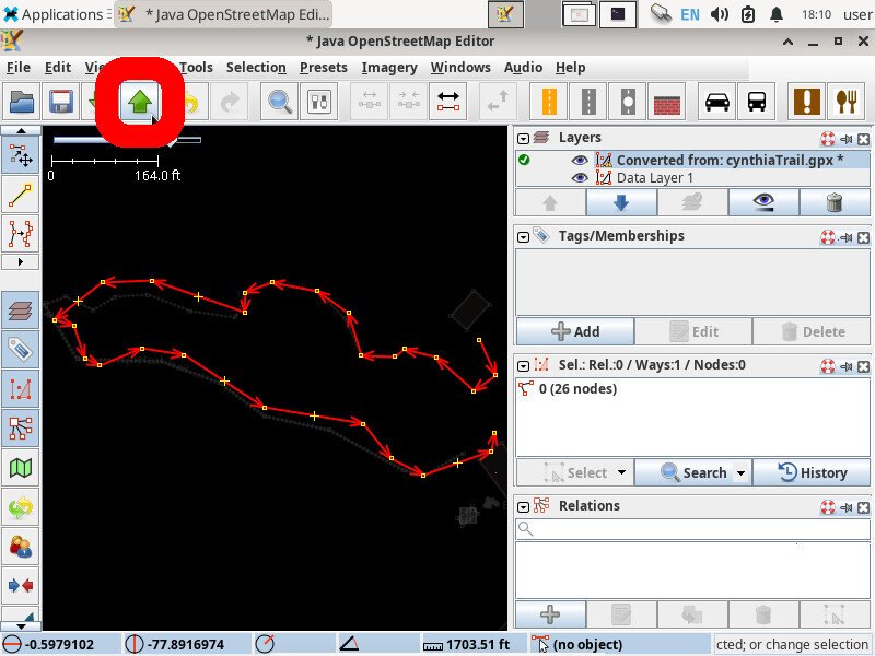
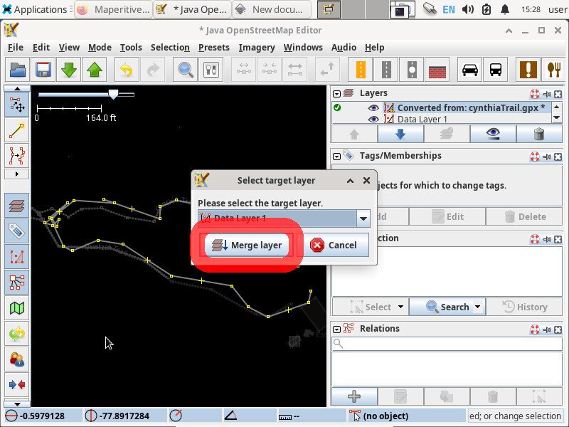
Finally, let’s export this data (our path and the downloaded OSM nodes/paths) from JOSM. We could either export each layer separately, or we could make our lives easier by mergeing both layers into one before exporting both layers as a single .gpx file.
To merge the layers, click Edit -> Merge layer
There’s only two layers, so go ahead and click “Merge layer” again
-

- Edit -> Merge layer
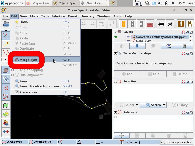
-
- Click “Merge layer”

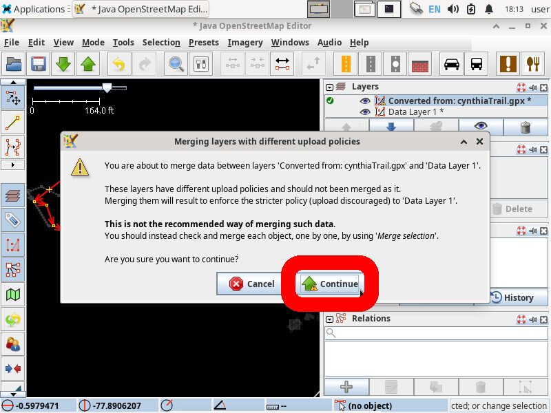
We’re just merging & exporting this for local use (not for upload to OSM), so go ahead and click “Continue” on the warning
-

- Click “Continue”
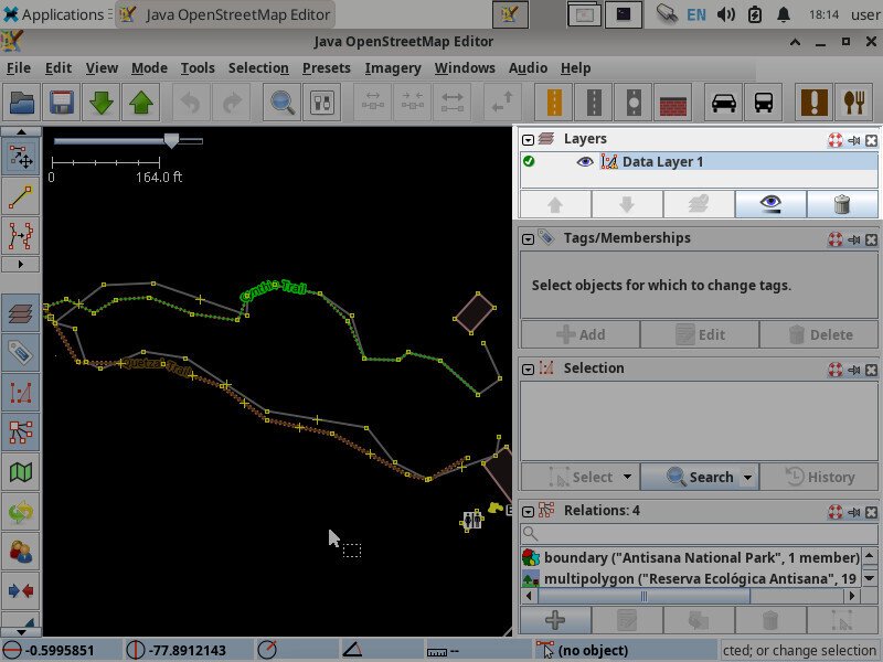
-

- Note that we now only have 1 layer
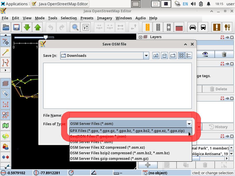
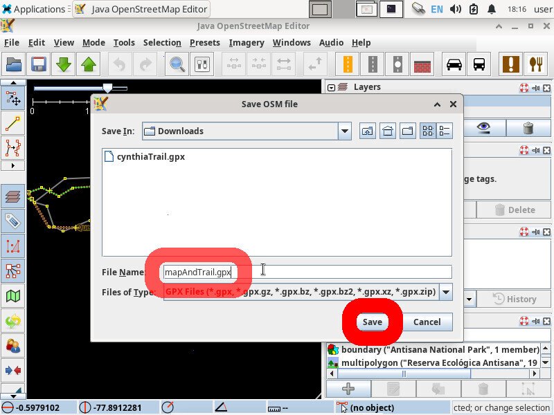
Now, to export the nodes and paths from JOSM, click File -> Save As
We’ll want to save this as a .gpx again, so change the filename from .osm to .gpx
-
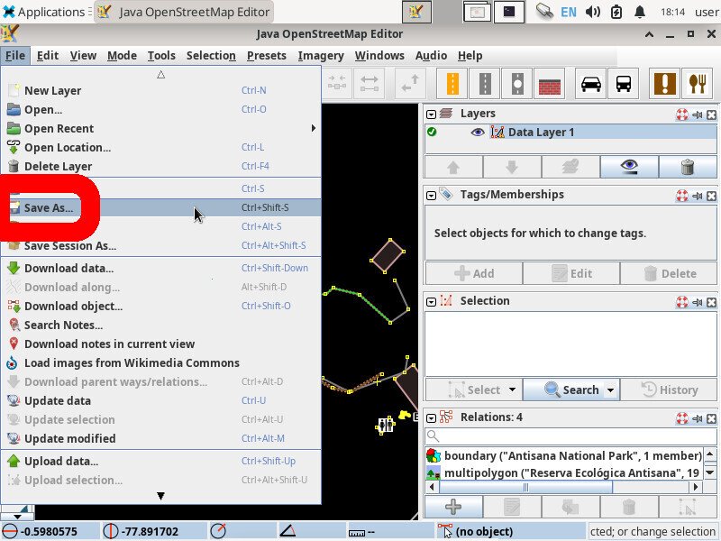
- File -> Save As…

-

-
Change from ‘
.osm‘ to ‘.gpx‘
-
-
Save the combined data to a new ‘
.gpx‘ file

Downloading Contour Data
Next, let’s download the SRTM-derived relief data from viewfinderpanoramas.org
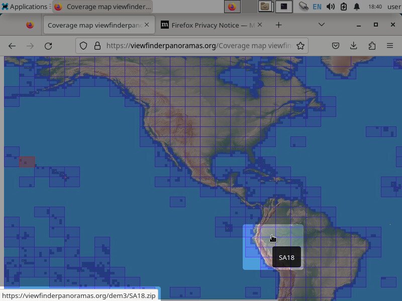
Click to download the tile where you’re mapping. We download eastern Ecuador, which is ‘SA18.zip‘
The data is split into .zip files projected onto a map. Just click on the square of the map that contains the area that you want to map to download the corresponding .zip file.
You might need to download more than one file. The country lines are absent, so we downloaded both ‘SA17.zip‘ and ‘SA18.zip‘.
Generate the Vector Topo Map
Next, let’s use Maperitive to line-up our .gpx tracks exported from JOSM and generate some vector contour lines around it.
Install Maperitive
The best tool I found for generating an SVG from contour data is Maperitive. Unfortunately, Maperitive was designed for Windows. Fortunately, it does run fine in Linux. You don’t even need to install wine. Just install the mono package.
First, install the prerequisites.
sudo apt-get install mono-complete
Now download, extract, and launch Maperitive
⚠ WARNING: Downloading and installing software outside of
aptis not recommended. By default,aptwill cryptographically verify the authenticity of everything that it downloads before installing it. Whereas downloading and running a script from the Internet (even with https) could lead to you installing malicious software.If you must download software without verifying its authenticity (eg with PGP signatures), then you should at least check it with 3TOFU.
Moreover, Maperitive is closed-source software that hasn’t been audited (and cannot easily be done-so because the author won’t release the source code). Security researches can’t, for example, read the sourcecode of Maperitive to determine if it’s installing a keylogger to steal your passwords or monitoring your Internet activity to sell to data brokers. In practice, most closed-source software does malicious things, so you probably should only install Maperitive in a sandboxed VM that you delete after you’ve printed your map.
# WARNING: this is not safe and could download malicious code!
mkdir Maperitive
cd Maperitive

wget http://maperitive.net/download/Maperitive-latest.zip
unzip Maperitive-latest.zip
cd Maperitive

# create data dir for contours .hgt files
mkdir -p Cache/Rasters/SRTMV3R3/

# allow script to be executable
chmod +x Maperitive.sh
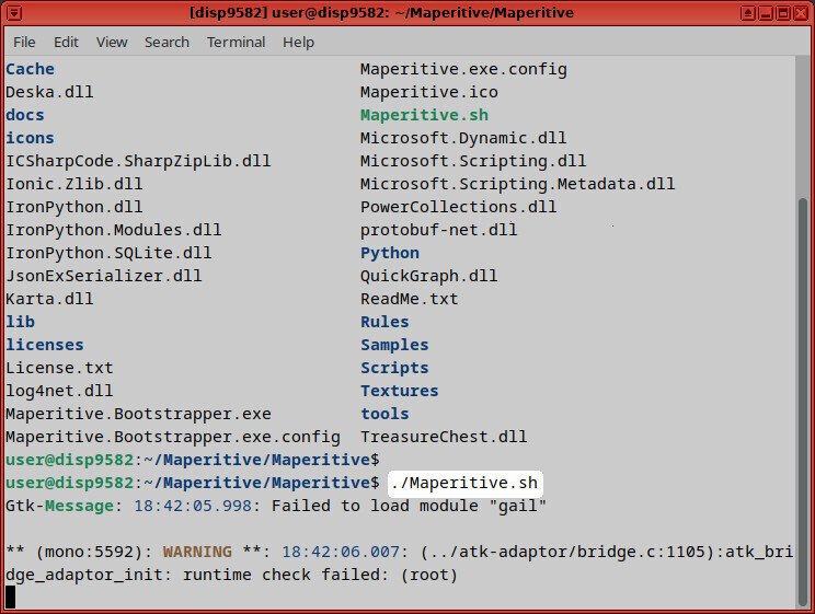
Finally, you can open Maperitive in linux by executing the Maperitive.sh script
./Maperitive.sh
-

-
Launch Maperitive by executing the
Maperitive.shscript from the command-line
Import Contour Data
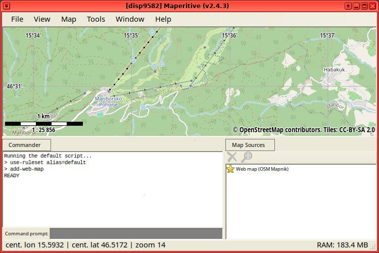
Maperitive is a powerful piece of software. It has a GUI, but most options (and parameters for commands) can only be accessed by the command prompt.
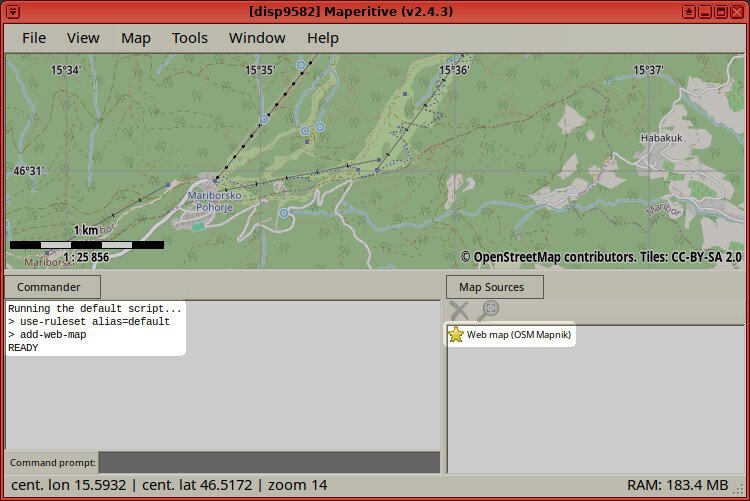
When Maperitive first opens, you can see that the `use-ruleset` and `add-web-map` commands were executed on startup.
Mapertive has the ability to import its content data from several distinct DEM Sources (Digital Elevation Models).
By default, Mapertive is set to use the US government’s SRTM source, but I’ve never had that work for me (and it’s not just me). That’s why we downloaded the Vector Topo data above.
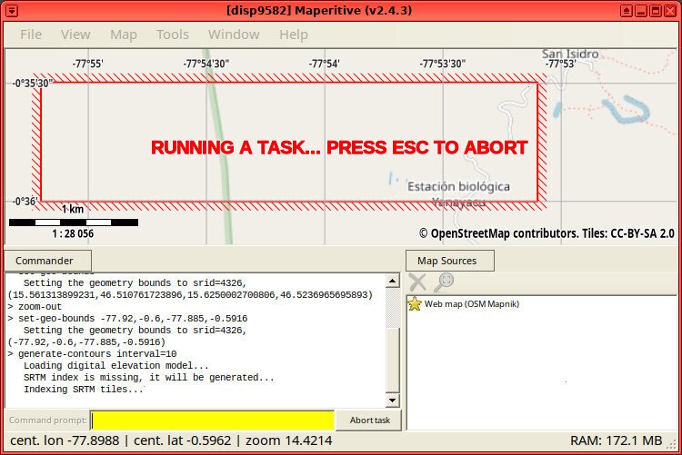
# by default, Maperitive fails to download the SRTM data; use Vector Topo .hgt files instead
> generate-contours
   Loading digital elevation model...
   SRTM index is missing, it will be generated...
   Indexing SRTM tiles for the 'Australia' region.
   Error downloading SRTM data (reason: The remote server returned an error: (404) Not Found.)
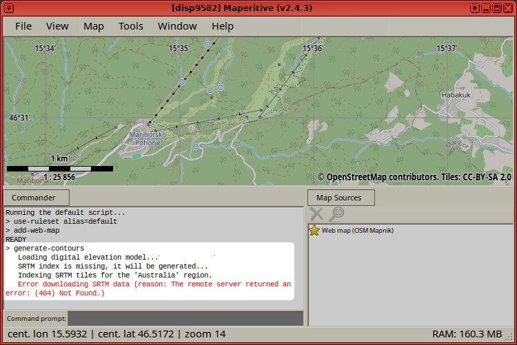
Mapertive fails OOTB to download SRTM data for contours
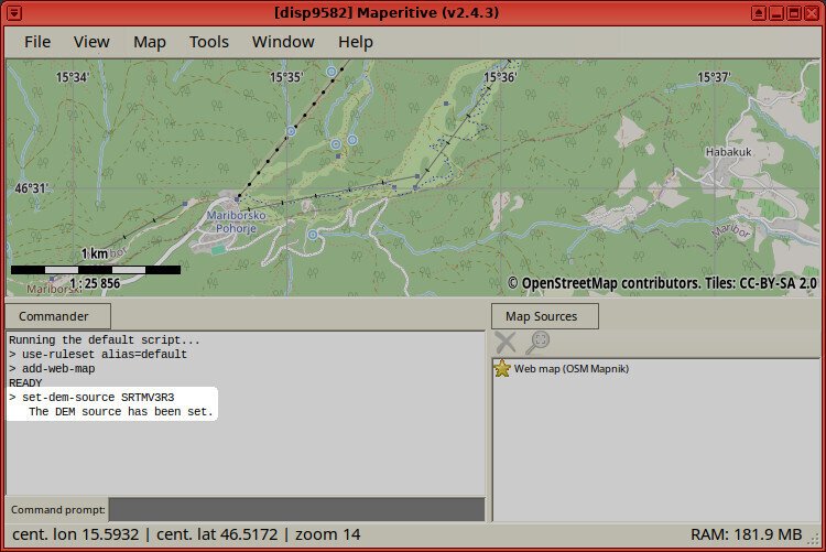
Before we can import the Vector Topo data into Maperitive, we have to create a new DEM source. We do that with the set-dem-source command.
Execute the following command inside the Maperitive GUI’s command prompt:
set-dem-source SRTMV3R3
-

- Change the directory for the SRTM data
-
-
Add the
.hgt(SRTM data) files (downloaded from Viewfinder Panoramas)

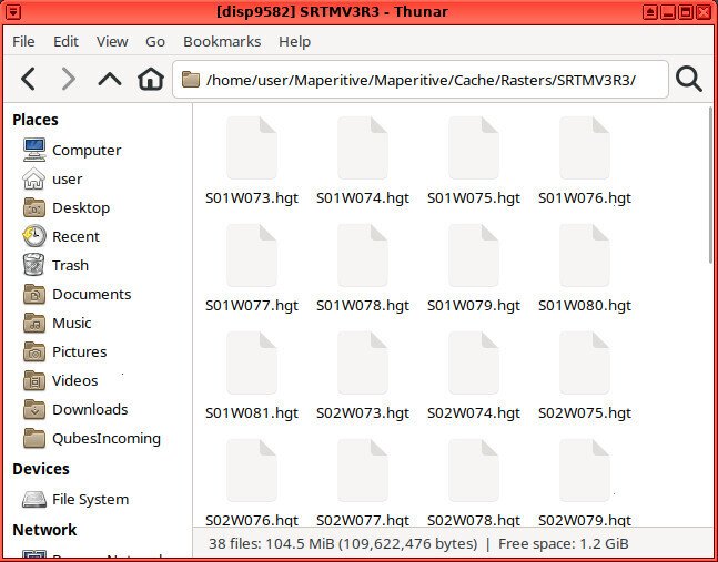
After executing the above command in Mapertitive, we must extract the .hgt files from the Vector Topo .zip file(s) and paste them into this Maperitive/Cache/Rasters/SRTMV3R3/ folder.
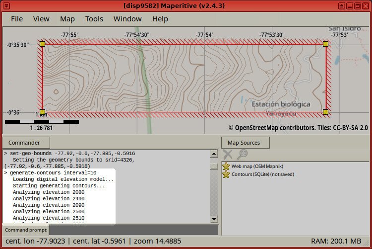
Set Geometry Bounds
Above the command prompt in Maperitive is a map. Left-mouse-click-and-drag to pan. Zoom-out and zoom-in to the area you want to map with the mouse wheel (or touchpad scroll gesture). Then click Map -> Set Geometry Bounds to draw a red-box around the viewbox to select the area that you want to map.
Zoom-out a bit, and you can see the bounds of the red box. You can click the yellow corners of the red box to resize the box as needed.
-

- Map -> Set Geometry Bounds
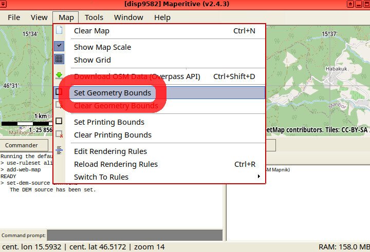
-
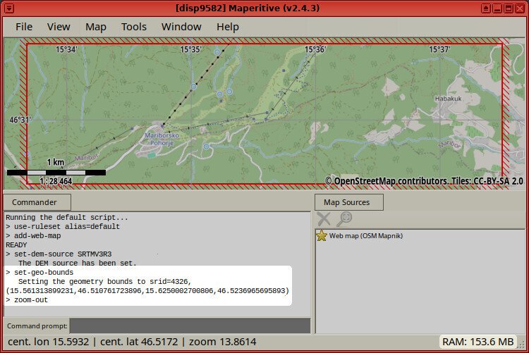
- Zoom out to see the red bounding box

Note that the command prompt window shows the `set-geo-bounds` command that it executed when you clicked “Set Geometry Bounds” – including the parameters that define the bounds of the box.
Maperitive is a software that’s dealing with some big data sets. In fact, the amount of memory that it uses is literally always visible in the bottom-right corner of the app. It’s quite possible that you might, at some point, kick-off a processing command that exhausts your system’s memory, causing Maperitive to crash. For this reason, I think it’s super helpful that all Maperitive actions can be entered as a command. This allows you to write a set of idempotent commands that you can execute in Mapertivie, to quickly return to where you were before it crashed.
I recommend spending a few minutes manually executing the set-geo-bounds command – changing the parameters bit-by-bit until the box meets your needs. Then write-down the full command so you can easily paste it into Maperitive on a subsequent run to draw the same bounding box.
For the purpose of this guide, we’ll be using the following box:
set-geo-bounds -77.92,-0.6,-77.885,-0.5916
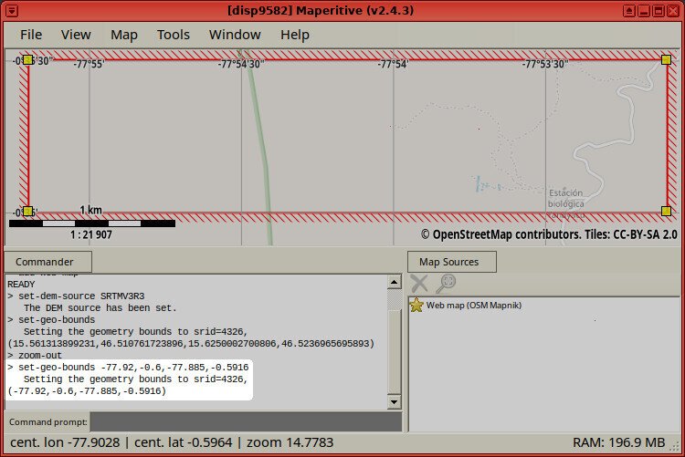
We can specify the geo-bounds on the command-line for precision and reproducibility
After executing the above command, you’ll have a red box drawn around the Yanayacu Biological Station and the surrounding Antisana National Park near Cosanga, Ecuador. You may need to zoom-out and pan to South America to view the geo-bound red box.
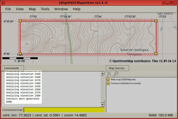
Generate Contours
Finally, we can actually generate our contour lines. You can do this by Tools -> Generate Relief Contours
-

- Tools -> Generate Relief Contours
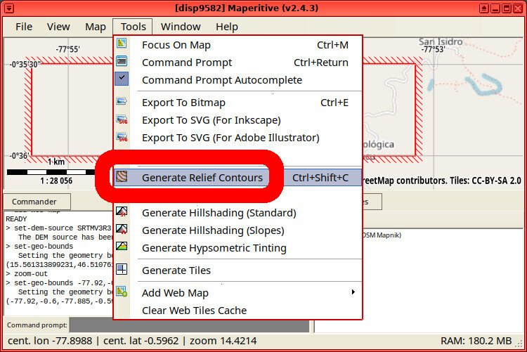
-

- Generating Contour Lines in Maperitive
Or you can generate contours with the `generate-controus‘ command (which has the added benefit of letting us set the coutour line interval).
generate-contours interval=10
-
- Generated Contour Lines (1/2)

-

- Generated Contour Lines (2/2)
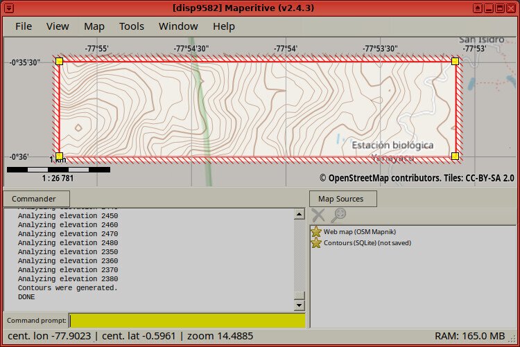
Generate Hillshades
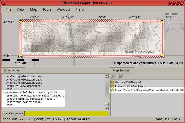
If you’d like, you can also generate hillshades. There’s a few different “methods” you can use. We’ll use the author of Maperitive (Igor Brejc)’s method generate-relief-igor with 1.25 intensity.
generate-relief-igor intensity=1.25
A few notes about this:
- The hillshades will look terrible and blocky in Maperitive; they will look fine once exported to
.svg - The hillshades will export as raster bitmaps, not vectors. But since they’re just semi-transparent gradients, it should look ok when scaled-up
-
- Generate Hillshades (1/2)

-
- Generate Hillshades with “Igor” method (2/2)

Customize Contour Lines
How frequently do you want a contour to be drawn? Every 50 meters? Every 10 meters? Every 1 meter? And how frequently do you want the text to appear, indicating the elevation of a given line? Every 100 meters?
You can control these settings in Mapertive with Rendering Rules.
Maperitive comes with a few different sets of Rendering Rules, which can be found in the Maperitive/Rules/ directory
user@disp4463:~/Maperitive$ ls Rules/
Default.mrules       Experimental.mrules  Hiking.mrules      urbanight.mrules
GoogleMaps.mrules    PowerLines.mrules    Wireframe.mrules
user@disp4463:~/Maperitive$
I found that I liked the detail of the contour lines provided by the Hiking.mrules rules, but that ruleset hid my GPX tracks for some reason.
The easiest way I found was to just edit the Default.mrules file, copying & pasting the relevant sections from the Hiking.mrules file back into the Default.mrules file. Then, the only other thing that I customized was to increase the font-size — because I wanted the elevation printed on the major contour lines to be visible when printed on A4-size paper, a posterboard, and even when a cheap printer with low DPI is used.
Here’s the two relevant sections as they originally appeared in Default.mrules
                contour major : contour[@isMulti(elevation, 100)]
                contour minor : contour[@isMulti(elevation, 20) and not @isMulti(elevation, 100)]
        target: contour*
                define
                        line-color : #7f3300
                        line-opacity : 0.35
                        curved : true
                if : *major
                        define
                                map.rendering.contour.label : true
                                min-zoom : 9
                                line-width : 11:0.1;11.9:1;12:2
                                font-size : 10
                                font-style : italic
                                font-weight : normal
                                text-halo-width : 35%
                                text-halo-opacity : 1
                                text-halo-color : #F1EEE8
                else
                        define
                                min-zoom : 12
                                line-width : 1
                draw : contour
Here’s as they appear in Hiking.mrules.
                contour major : contour[@isMulti(elevation, 50)]
                contour minor : contour[@isMulti(elevation, 10) and not @isMulti(elevation, 50)]
        target: contour*
                define
                        line-color : #7f3300
                        line-opacity : 0.6
                        curved : true
                if : *major
                        define
                                map.rendering.contour.label : true
                                min-zoom : 12
                                line-width : 11:0.75;13:1.25;15:2
                                font-size : 10
                                font-style : italic
                                font-weight : normal
                                text-halo-width : 35%
                                text-halo-opacity : 1
                                text-halo-color : #F1EEE8
                else
                        define
                                min-zoom : 13
                                line-width : 0.65
                draw : contour
And here’s a diff of the original Default.mrules file vs the one after my edits.
user@disp4463:~/Maperitive$ diff Rules/Default.mrules.orig Rules/Default.mrules
126,127c126,127
< 		contour major : contour[@isMulti(elevation, 100)]
< 		contour minor : contour[@isMulti(elevation, 20) and not @isMulti(elevation, 100)]
---
> 		contour major : contour[@isMulti(elevation, 50)]
> 		contour minor : contour[@isMulti(elevation, 10) and not @isMulti(elevation, 50)]
1352c1352
< 			line-opacity : 0.35
---
> 			line-opacity : 0.6
1357,1359c1357,1359
< 				min-zoom : 9
< 				line-width : 11:0.1;11.9:1;12:2
< 				font-size : 10
---
> 				min-zoom : 12
> 				line-width : 11:0.75;13:1.25;15:2
> 				font-size : 5120
1367,1368c1367,1368
< 				min-zoom : 12
< 				line-width : 1
---
> 				min-zoom : 13
> 				line-width : 0.65
1375c1375
< 		draw : line
\ No newline at end of file
---
> 		draw : line
user@disp4463:~/Maperitive$ less Rules/Default.mrules.orig
Add .gpx
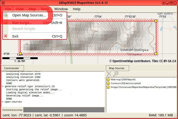
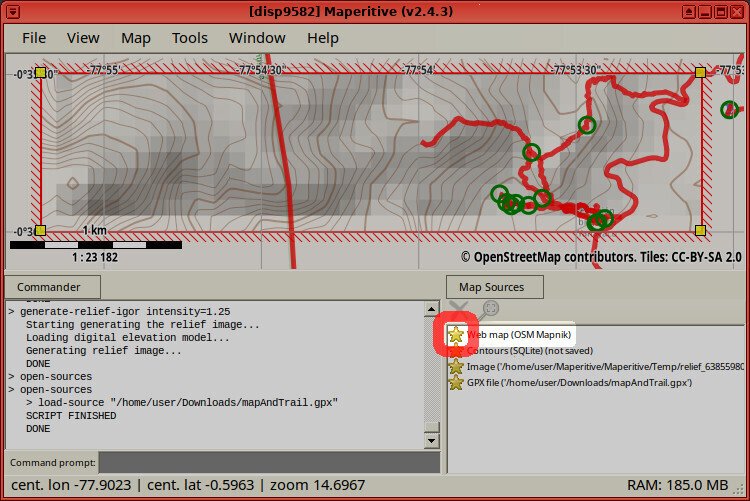
To overlay the trace of your walk along the trail on the map, open your .gpx file in Maperitive.
-

- File -> Open Map Sources…
-

-
Open the
.gpxfile from JOSM
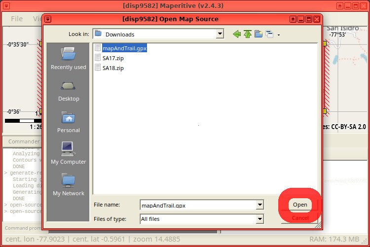
Go to File -> Open Map Source, then browse and select your .gpx file.
Export .svg
Finally, we want to export all of this data from Maperitive to a .svg file.
Note that some data in Maperitive can not be exported as a vector. Layers like Web Maps are loaded as rasterized tiles.
Before you export to your .svg file, you probably want to go through each of your current Map Layers. We only want the following layers:
- Contours(SQLite) – Our contour lines layer, generated with the
generate-contourscommand - Image(‘…Maperitive/Temp/relief…png) – Our hillshades layer, generated with the
generate-relief-igorcommand - GPX file… – OSM data from JOSM and the trace of our walk on the trail
You may see additional layers that Maperitive added automatically, such as a “Web map“. You probably want to hide these layers before exporting the .svg file. Hide them by clicking the yellow “star” icon next to the Map Layer’s name.
-
- Click the “golden star” icon to hide the “Web map” layer

-
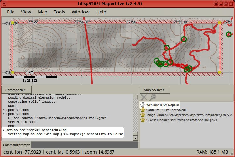
- Hidden layers have a “grey star” icon

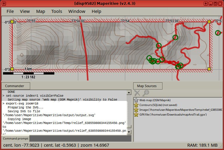
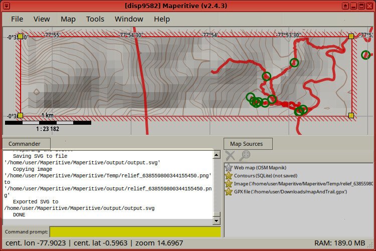
The Maperitive command to export the map to an .svg file is export-svg. This command takes many arguments. We’ll be using it with the zoom argument.
export-svg zoom=18
The above command will output an ‘output.svg‘ file, located in the ‘Maperitive/output/‘ directory.
Note that we chose zoom level 18. The bigger the number, the more “zoomed-in” and the bigger the file. You may want to increase or decrease the zoom level to meet your needs, but I found that 18 worked well for our map.
-
-
Export
.svgwith vector contour lines from maperative at zoom level 18

-

- Vector topo map exported
Finalize in Inkscape
Rather than open the .svg file in inkscape, I recommend:
- Create a new inkscape document
- Set the page size of the inkscape document to the actual dimensions on which you plan to print your map (on paper), and
- Import the Maperitive-exported ‘
output.svg‘ file into the new inkscape document
Create Inkscape New Document
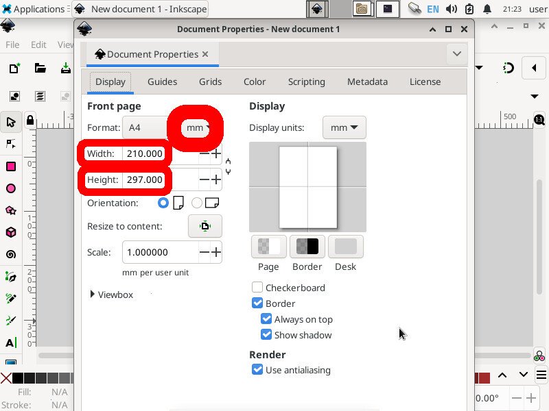
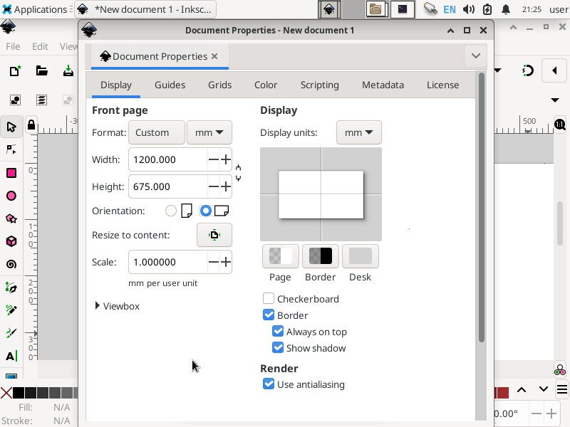
Download, install, and open a new inkscape document. Go to File -> Document Properties.
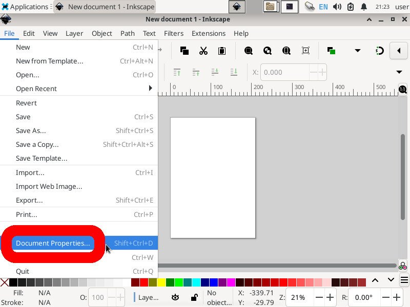
File -> Document Properties
We decided to make a map 1,200 mm x 675 mm (that’s 1.2 meters wide by 0.675 meters tall), so we set the document units to mm, set the width to 1200.000, and set the heght to 675.000
-

- Set the width and height to the actual dimensions on which you plan to print your map (on paper)
-
- Our map will be 1.2 meters wide x 0.675 meters tall

Import Maperitive .svg into Inkscape
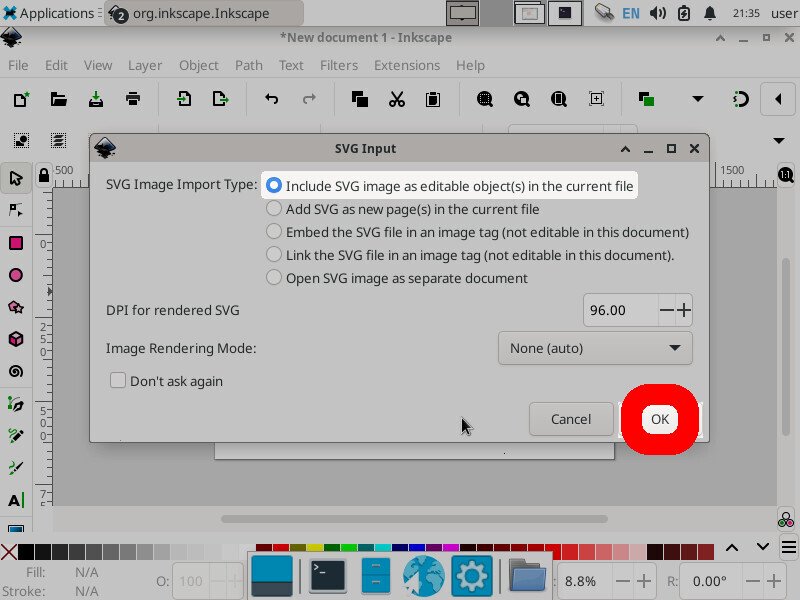
After your page dimensions are set correctly, go to File -> Import..., and browse to the ‘Maperitive/output/output.svg‘ file that you produced above. In the pop-up that follows, click “Include SVG image as editable object(s) in the current file”
-

- File -> Import…
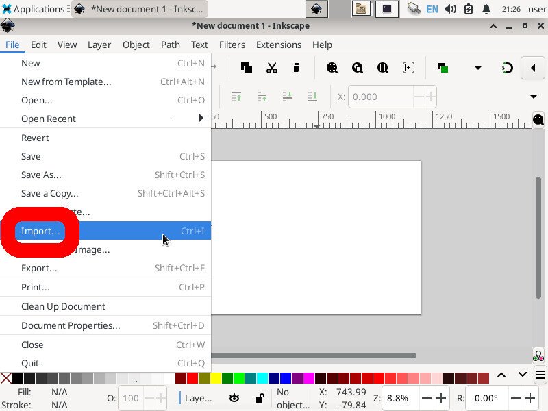
-
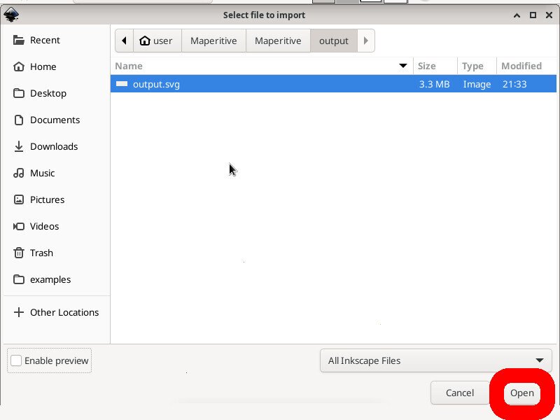
- Select the file exported by Maperitive

-

- Choose “Include SVG image as editable object(s) in the current file”
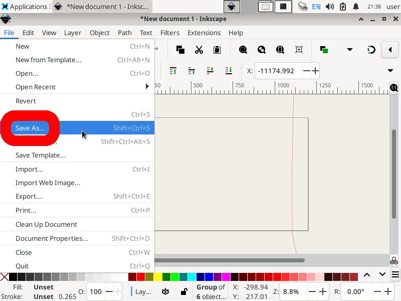
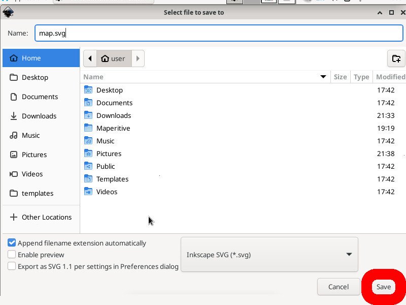
At this point, you probably want to save your document before continuing — working with large map files have a tendency to crash programs. Go to File -> Save as... and save this new inkscape document as an .svg file somewhere on your computer.
-

- File -> Save As…
-

- Protip when working with big files: [1] Save early, and [2] Save often.
Scale
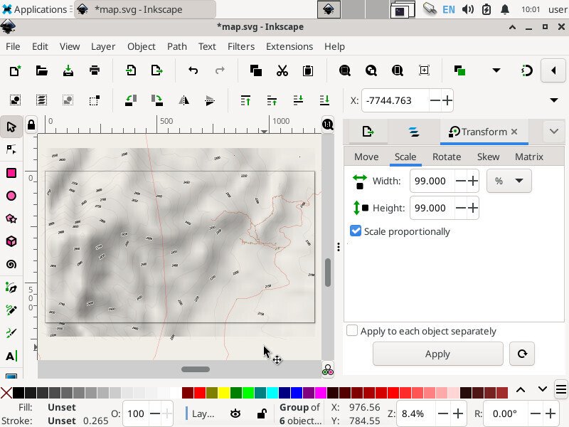
If your map is too big, scale it down to the size of your document.
-
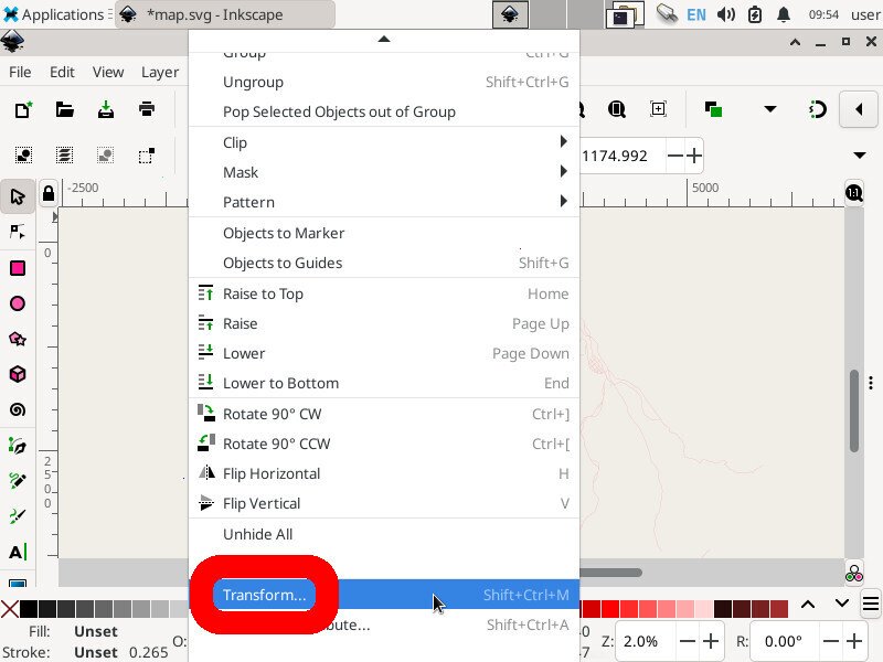
- Object -> Transform…

-
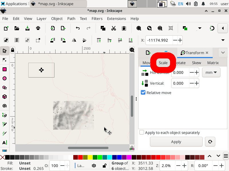
- Click the “Scale” tab

-
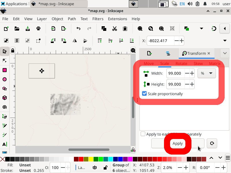
- Set the width & height to 99%. Press “Apply” over-and-over as-needed to shrink the map.

If your map is too small, you might want to consider re-exporting a new output.svg file from Maperitive — but this time use a slightly higher number for your ‘zoom=‘ parameter.
ⓘ Note: Maperative has a maximum zoom level, such that if you keep increasing the ‘
zoom=‘ parameter, the output file won’t get any bigger.You can increase the maximum zoom level in Maperitive using the set-setting command. For example, the following command will increase the maximum zoom level to 21
set-setting name=map.max-zoom value=21
When your map looks slightly larger than your page, click-and-drag the map layer so it’s positioned directly over your page, and then continue to shrink it until it fits into your page as-desired.
-

- Click-and-drag the map layer over your page
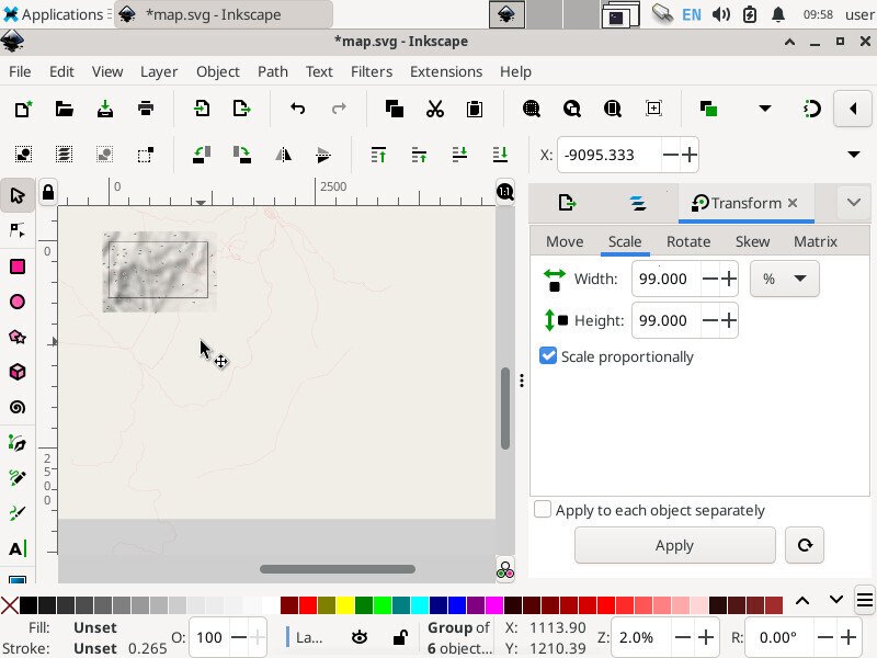
-

- Continue to shrink & move as-needed
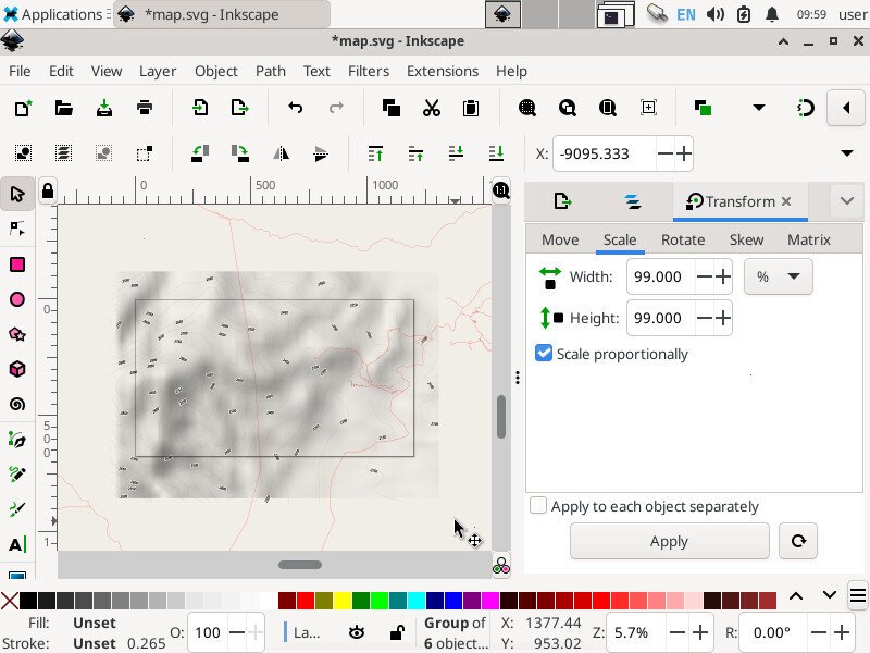
-

- Our map is the same width as our page
Customize Lines and Stroke
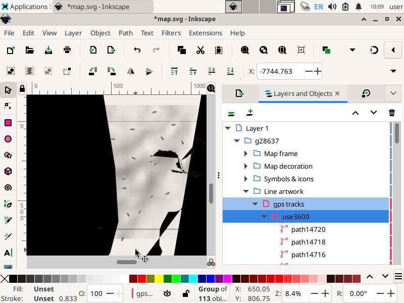
The .gpx data that you exported from Maperitive (and also the contour lines) should appear in the Inkscape Layers and Objects tab under the a sub-group named “Line artwork”.
-

- Layer -> Layers and Objects…
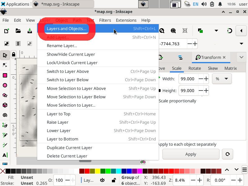
-
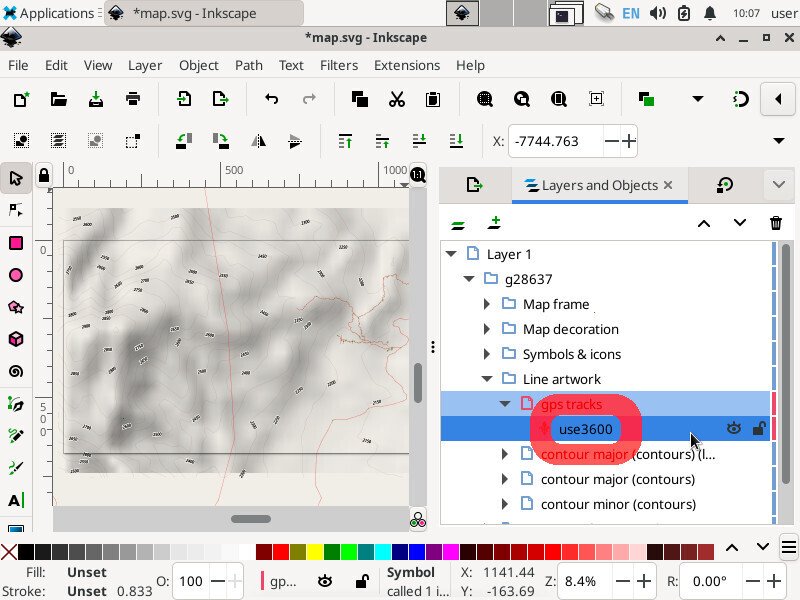
- Select the layer under “Line artwork” -> “gps tracks”

-
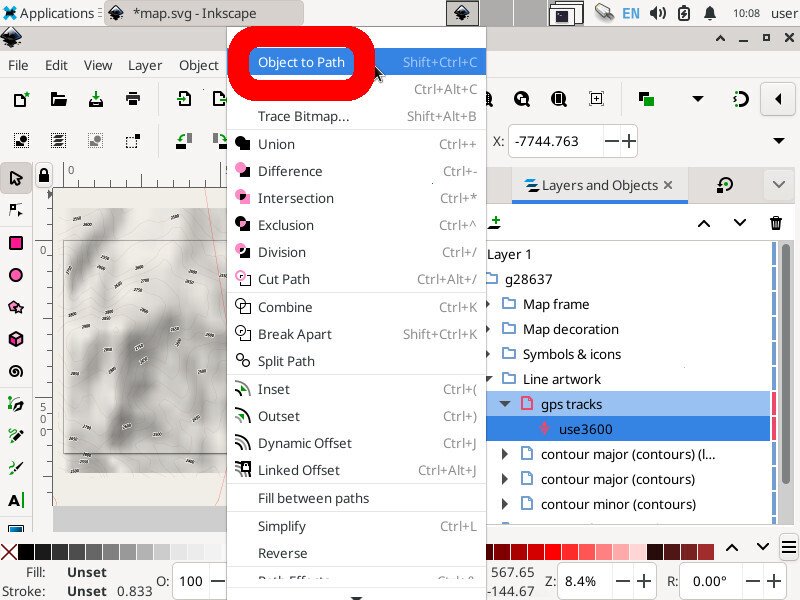
- Path -> Object to Path

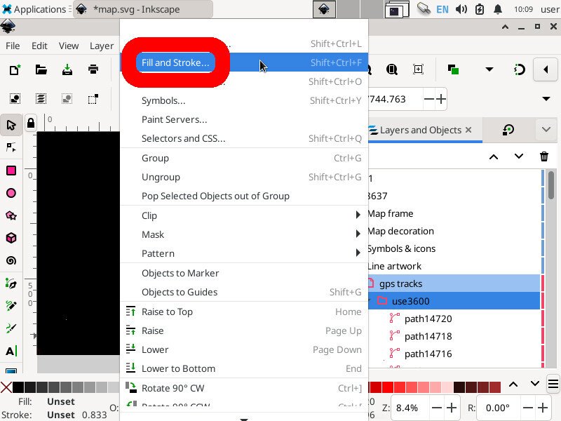
If it appears as a single large, un-editable shape, you may need to
- Select the object in the layer list
- Click Path -> Object to Path
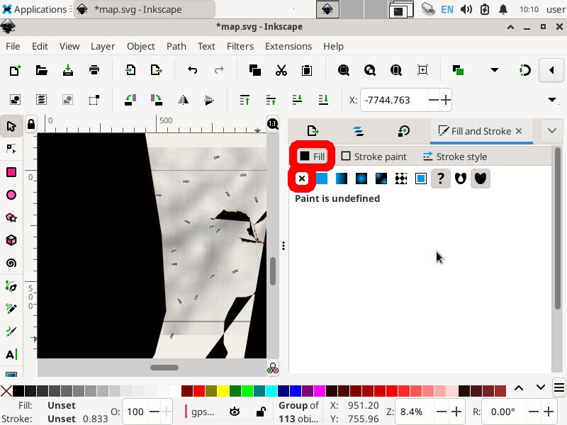
- Open the Fill and Stroke dialog by clicking “Object -> Fill and Stroke”
- In the “Fill” tab, click the “X” icon to select “No paint” for the path’s Fill
-

-
The layer is now a group, with many paths under it. This allows us to select (and modify) individual lines from the
.gpxfile
-

- Object -> Fill and Stroke…
-

- Fill -> No Paint
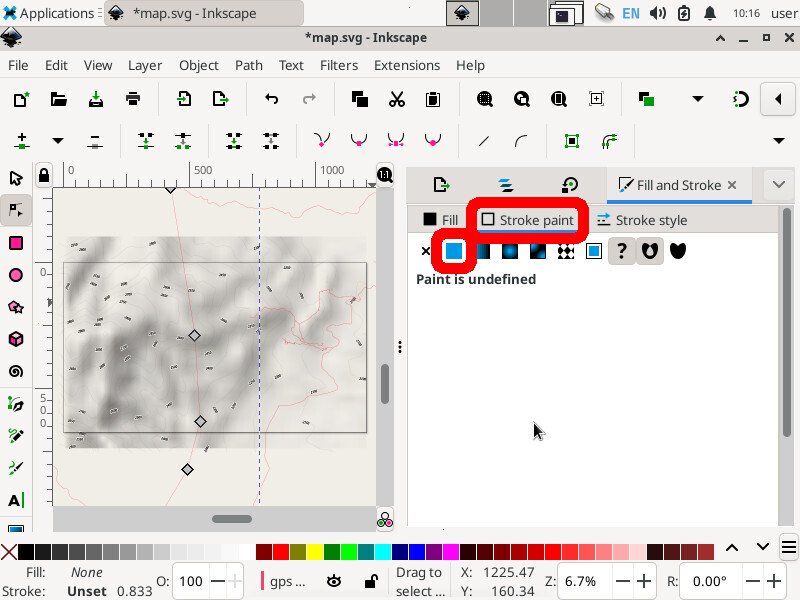
You should now be able to click on a given line segment to edit its appearance. For example
- Click on the line that traces your path following the trail
- In the “Fill and Stroke” dialog, click on the “Stroke paint” tab
- Click on the “Flat color” icon
- Choose a different color on the color wheel
- In the “Fill and Stroke” dialog, click on the “Stroke style” tab
- Change the “Width” to “10.000” mm
- Change the “Dashes” dropdown to a solid line or a style of dashes to trace the line
-
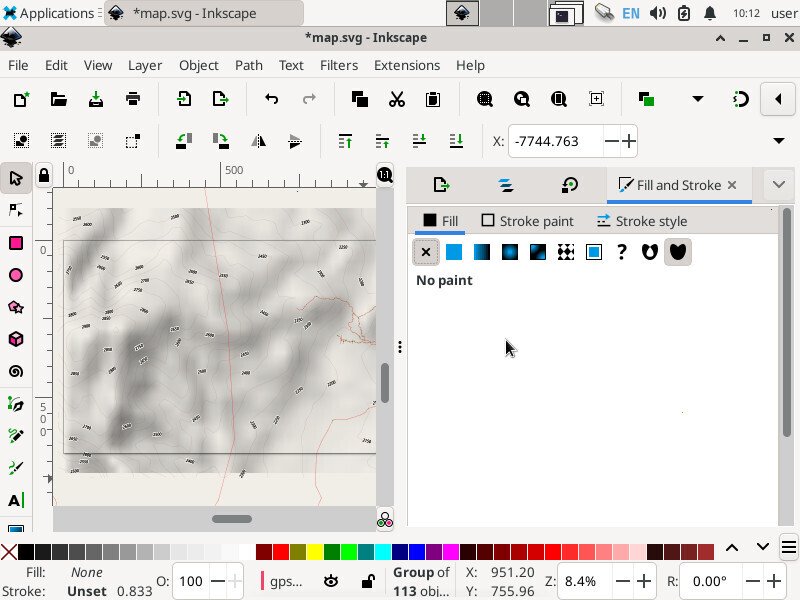
- Changing “Paint is undefined” to “No paint” fixes the black fill chaos

-

- Stroke paint -> Flat color
-
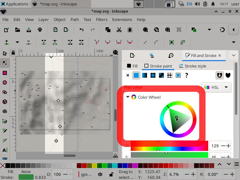
- Select a color on the Color Wheel to change the color of the selected line.

In this example, we change the stroke of the “national park boundary” line to be thick, green, and dashed.
-

- Change the “Width” and “Dashes” options to change the selected line’s stroke style.
-
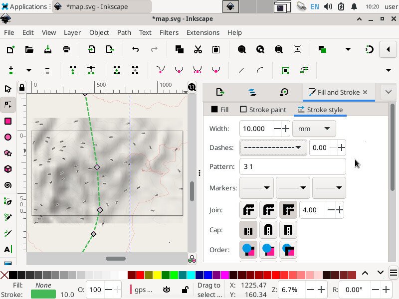
- We changed a “thin red solid line” to a “thick green dashed line”.

In addition to changing the color, thickness, and stroke pattern of the lines, you can also hide some lines that you don’t want to appear.
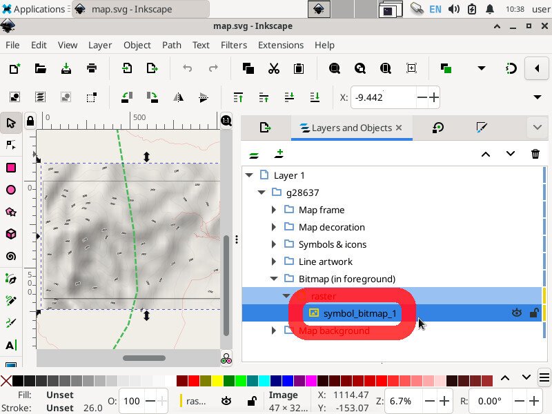
Embed raster images
At this point, the hillshades in the svg are referenced externally. That is to say, if you send just the .svg file to a colleague (without the externally-referenced .png file), then inkscape will show a big red X instead of the hillshades gradient.
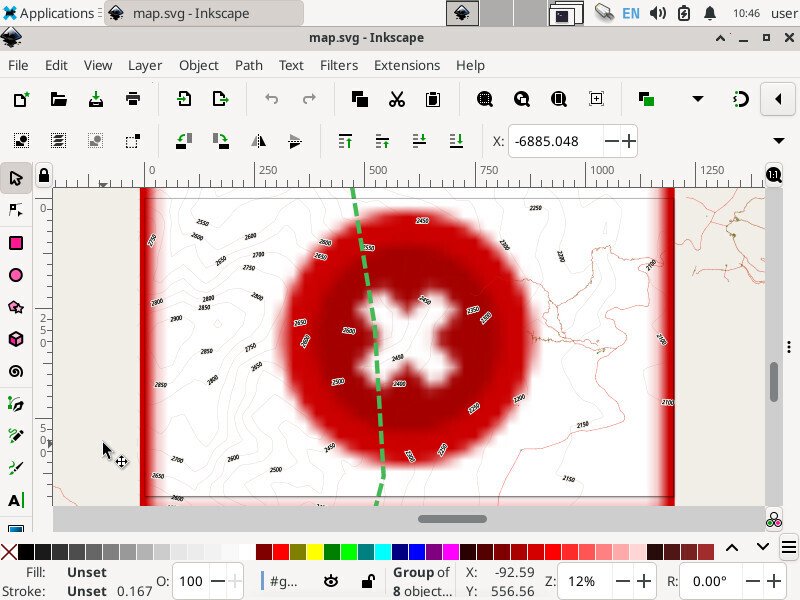
Inkscape displays a large red “X” if it can’t find the externally-referenced raster image
<!-- externally-referenced hillshades png file -->
<image
   id="symbol_bitmap_1"
   width="47"
   height="32"
   transform="matrix(154.68,0,0,-157.29,41259.53,22405.23)"
   xlink:href="../../../Maperitive/output/relief_638543156646443800.12.png" />
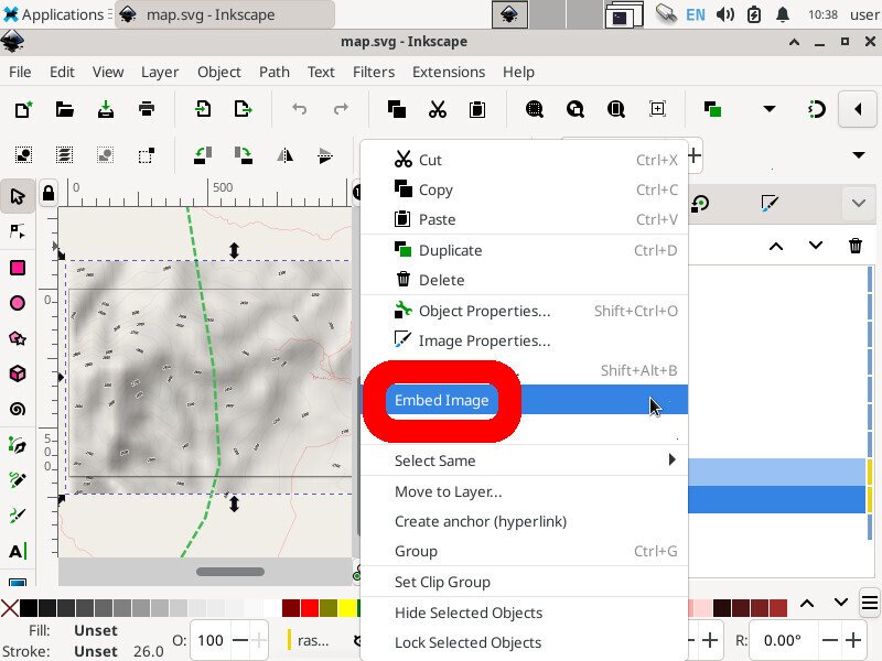
To prevent this issue in the future, go ahead and embed the hillshades data directly into the .svg file (in our map, it was only 2 KB) by right clicking on the raster layer and selecting Embed Image
-
- Right click on the raster layer

-
- Click “Embed Image”

<!-- embedded hillshades png data -->
<image
   id="symbol_bitmap_1"
   width="47"
   height="32"
   transform="matrix(154.68,0,0,-157.29,41259.53,22405.23)"
   xlink:href="data:image/png;base64,iVBORw0KGgoAAAANSUhEUgAAAC8AAAAgCAYAAACCcSF5AAAABGdBTUEAALGPC/xhBQAAAAFzUkdC
AK7OHOkAAAAgY0hSTQAAeiYAAICEAAD6AAAAgOgAAHUwAADqYAAAOpgAABdwnLpRPAAABmxJREFU
WIVlmFuT20QQhT9Jvq7tTbK7JKSgCAVvUMUb//9H8MIDL6SKIgnJ7np90cryhYc5x90YValsaWZ6
Tt9O96iiXL8CNfACaIAD8BH4HfhKdwM8a6wGhnp+BhZAD3zS+HfALbAB/gGWaV2l+6Q1B+Co51p4
Dnoe6PmosUP6XzUavAOuBGKozX4D3gAvgT2wA8bauBPoXmvvJHgreWNgJABo/f4CZK3/nuOrEYZK
z6ekjOdWQGPNdsBTmvQFeAdMNdYmCxx0X0vIVkqv9X4iAJ3WTGSYLq0nWTV7wrIHkmHjOhqsQJ3B
X2twLQvNgZ+16G/gvcZHGh9qg6UA9VJyk4BtBeoVxXvtBQB7ASJc/GwlDNyGq/RcAfUgLa60wUkg
X8pqddroGlgJdKf5NcVTbVLM+dFK1kxrT1Jyn/bNoAzySFwet1In7XFskpCdBg3qjuIBu2xCieUn
ShLaWq2F6d2tnlspYMWP/B8YhCcMMFvXzw4rYwU42fJdGlxr8RL4kRISRyIv1gLXa/47ipfeS/Bc
768SgF6K29JmHl8HzfW7iggdzx0QoXQChgZ/Q3GlJ4+BP4G3AvuXxk/pdwO8FtixFB5TktyWbAR2
KGWOSUafrJovY3ICm5kGBBn0wMFh8zXF+jOC7r5QWGSkzZ3QTwJ+pXmesxSQeQL+TMmRRhtPBcJx
PCS8kem00bwBwe+7dLfAzlo+E9Tk+LegqQA2AjIUWDOKmeZZv5+1bkIUlVbrR3pveU5gz8sE4igw
DoeV8+Ec840sNhLYXhs4zhbAtxL0BxEOFrTS8ygpvtKzc8DxbKU6KW9rovkey4ltRQdE8h5zfI0p
DHOSpQZEYn7S/42eve6WSO6ZFO+Isl8Tcdqk556g5x1BGC5QI8nP1j9d3GeqNCW+EQgXn7eyekeU
/54o4a/1/kEyZoT7DcbJaW5fSAH3Ni1RjR0aI4L3d5pnNjy3CbYglGR81sIFkUAzoqL2mvOZiFtX
2E7zOoIdfG3SnDsKtZqhfGXvWBG0LnvKiVx5A2+6FqgxUSknBAstgPs0viSK1JiIZ9Oiw6fTuhUl
1KaEhyba18asCHp1c7fVb27aGms+lnWmRJ+zleBvJGxDcaGB1gLvJF9QQuea0lr7zuFhYwyIVsKG
2xEUeSU5w+SZIxf5lN22BR4FDP0/CABaaFdOiVh+pTVOtgPRhWYedx7Ysq7ctqar7FQyXThNHq4F
Dp9zkXISNrLwI/AhKbAlXLeQQnu9G+r/PSUXHikJbPq0u6e6r/hv1Wz0bkDJJyfkjXCtk7Wz8nuD
n1Hc70x3XFUCtqFUVrt6LKFLrTfwPZHEDpclJSTcodZaf0NJ3lz6V1L+SdZ3buQ+x6xzpspbovNz
vOUuzlWyJcrzUrdbgKMAjYmC4pbCyUqab1Zz5R1pLM99KZk2phvEntTPu+01JU2lvRPJ81yq1wnc
KlnW1nWYuKzvtGZHHCPdMruxq4jG7kDxZAv8JINuiMK5J51h3xFuv5LARwFzgXB85hOQ6dXrZno/
puRFZqZnAXggkt0t9pY4vLjtzfE+11jOo3Nv870GPhJ0lFtVU1jus92TONzcq7TpnVliIQU+EO2F
mYgLWTZSbh9cqFylh6Qi1QA/yBKO7QnRY/jX9Gb+HRAx7gLlyvxAkIAL3Z0sXCUZbsrq9HvuHIlz
hkGfPe+w+YX4xLEk6GtLxK17FVvUVdbs4ZOTrdQRse1zp+nSlxOwJcLV14ESZhXlO9CQEh3uOE/5
u81rCXggCkZL9CX5wLCnxLQPHjXRBnsD06J7/UryXWHz6cptxguiKasoeedEnsuY7jDPVDmguPWF
NrvXb55sq5t3JxSKdYu7ooSdY9qhZg/Ywl2SbYXatJfpE8ppzlR9TRx4DqQiNdHvTHdHcHg+splt
rLDzoiaqYJPeW1FbuUkyrVj+dOh8Mh1eGsOs1AG7/EVqpUlzop95IMp7vl19p0RfYzn+BOI6cExj
Pui4ffZnRIdTLozOGyt0Spbfk2LeWWxetVVNfZnb86e3OdH7++TUpXGfkvZEH+4zr5ssK3pDfCbc
E6crezR/rKqA6vIz255SrO4F+DZZ0Nb1YnO5n/Ocnjh1ndI7KN6ykv6+6QO3Q3CbrG4yMPjzF4bM
827Ccovg+HNH6Y1y0XLxcHEbpf9mFRuoo3jKiuXPIX1atyd6mYwvHwV3/wKDONhHv3UmWAAAAABJ
RU5ErkJggg==
" />
Export .png
When you’re satisfied with your map, you’ll want to export it as a raster image.
Unfortunately, .svg files render differently in web browsers (eg firefox), Adobe Illustrator, and Inkscape. Since your local print shop may not use the exact same software as you, it’s best to export it as a huge raster image.
Click File -> Export...
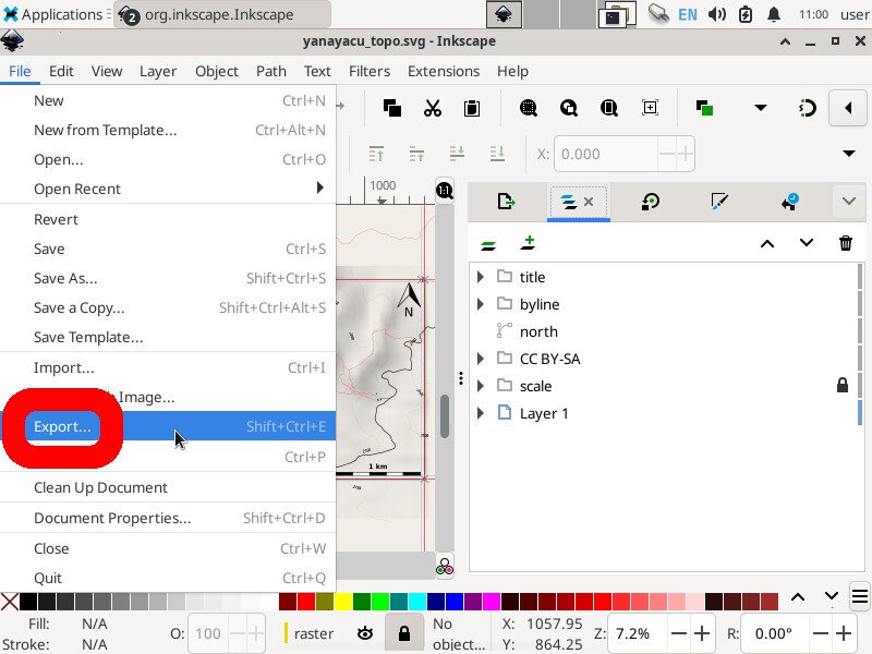
File -> Export…
Here you can only choose the size in pixels, not mm (you did set the document properties first, rather than editing the ‘output.svg‘ file directly, right?). If you’re going to print on paper that’s exactly the same size as the page size that you set in the document properties, then just export it at 300 DPI.
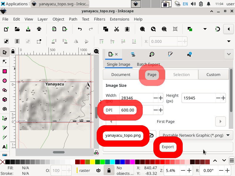
Ask the print shop what is the DPI of their printer
If you’re going to print it on paper that’s twice the size of your document, export it at 600 DPI.
If you’re going to print it on paper that’s half the size of your document, it should be fine to export it at 150 DPI.
You also might want to talk with your print shop before you export to .png. If their printer prints at 600 DPI, then you should export at 600 DPI instead of 300 DPI. They’ll know better than you or me what DPI the image should have.
For example, here’s the (A4-sized) topo map that I built for Yanayacu.

Final (raster) export, ready for sending to the print shop (source svg)
Note that I changed the stroke and thickness of the National Park boundary to be large and green, I changed the path of the road (downloaded from OSM data in JOSM) to be thick and black, and I changed my GPX tracks (recorded in OsmAnd and merged with the OSM data in JOSM) to be thin, dashed, and red.
The source .svg file for the above image can be found here
I also used this method to generate a simplified “trail map” of Yanayacu (without contour lines). The workflow was similar, except I didn’t generate contour nor hillshades layers in Maperitive before exporting as a .svg
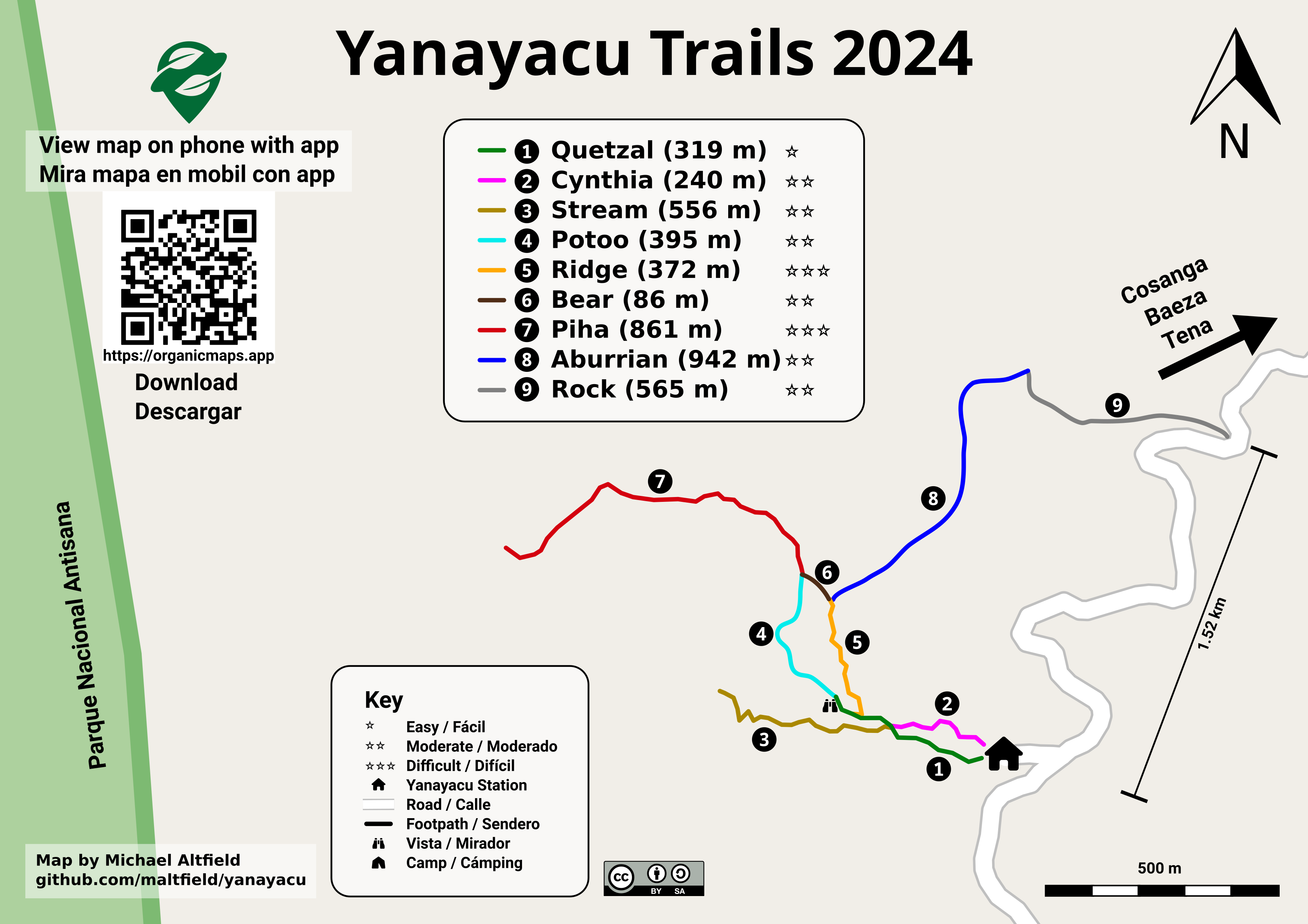
Yanayacu Trail Guide (source svg)
The source .svg file for the above image can be found here
Limitations
This section will outline some problems with this guide’s approach to creating vector-based topographical maps.
Raster Hillshades
While Maperitive can generate and export contour lines as vectors, it cannot generate and export hillshades as vectors.
The hillshades generated by Maperitive are a ~2 KB .png file that’s referenced externally by the ‘output.svg‘ file that Maperitive produces.
Not FOSS
The most glaring issue with this guide is that it heavily depends on Mapertive, which is a closed-source software designed in .NET. The author is actively hostile to the GPL.
Mapertive is closed-source software and its author is hostile to the open licensing.
The biggest consequences of this are:
- Some (exclusively FOSS-only) orgs cannot use the software in this guide
- If there’s a bug in Maperitive (and I found many), then the community cannot find & submit patches
- If the author stops developing Maperitive, then nobody can fork and continue development of Maperitive
- There isn’t a very large Maperitive community, partially because of the issues above
- Because the sourcecode cannot be viewed by security researchers, it could easily be doing something nasty, like recording all your keystrokes (including the passwords you type) and uploading a log of the websites you visit. The security risks are enormous. See #1 above.
One suggestion that I found was to use QGIS instead of Maperitive. If you know of any guides that describe how to use QGIS to generate vector-based topographical maps, then please link to it in the comments or email me.
Additional Resources
The reader may be interested in the following guides, as well.
- Creating the “Perfect” Hiking Map for Germany and other Countries by Hauke Voss
- Topographical Push Pin Map by Christopher Fisher
- Maperitive for laser cutting and 3D printing
Related Posts


Hi, I’m Michael Altfield. I write articles about opsec, privacy, and devops ➡


_(39680659444).jpg)
_Illustration.jpg)
Leave a Reply